Chapter 4 Sentiment Analysis
4.1 Definition of Sentiment Analysis
To explain sentiment analysis so a 10 year-old can understand: It is the process of analyzing a piece of text and to determine if the writer’s attitude towards the subject matter is positive, negative, or neutral. I am going to analyze the Berkshire letters to infer Buffett’s attitude towards the past results of the business and his outlook.
4.2 Setting Expectations
I want to set expectations before moving further. It would be great if we could use changes in the sentiment of Warren Buffett’s letters to predict movement in Berkshire’s stock to make millions of dollars. I can say with full confidence that this won’t happen. Sentiment will likely be a coincident indicator at best. What the sentiment score will represent is an “educated guess” of Buffett’s attitude, gleaned from his letters, concerning a mix of the performance over the past year and the outlook going forward. Given that the market is extremely efficient, any positive or negative performance over the past year as well as expectations for future performance will already be incorporated into Berkshire’s stock price. Therefore it is unlikely that the sentiment of Berkshire’s letters will influence it’s stock price. In fact, one could do a simple event study to see if Berkshire’s stock price has a meaningful change in the trading days after the letter is released. But since fourth quarter earnings are release simultaneously with the letter it would be difficult to disentangle the sentiment of the letter from the performance of the business (the latter of which should already be incorporated into the stock price anyway). Bottom line: my expectations are low and so should yours.
4.3 Sentiment Analysis Roadmap
In essence, natural language processing is really just math and statistics. Figure 4.1 shows the roadmap.
Figure 4.1: Roadmap for Sentiment Analysis
The process starts with academics or other investigators taking a subset of words and using some technique (manual, crowd sourcing or machine learning) to categorize them as positive, negative or neutral. The resultant list is the sentiment lexicon. The words in a corpus (in our case the 49 Berkshire letters) are matched against the lexicon and a sentiment score is generated for each word in the lexicon (note that not all words in the letters are in the lexicons and lexicons contain different words). Scores of the individual words in a given years’ letter are aggregated and and the result is a sentiment score for the letter for that year. The score is observed as it changes over time and inferences are made to account for the change in sentiment.
4.4 Limitations with “Bag of Words” Approach
As mentioned previously, word counting methods do not capture the relationships between words. They ignore order and context. For example, intensifiers have no effect, so that adding extremely, or very will not change the value. If you took two phrases as “We had a good year.” and “We had a very good year.” The intensifier would make the second phrase more positive but the lexicon just counts each instance of “good” the same. Also, negations have no effect, so the phrase, “It was not a good year.” would show as positive.
4.5 Toy Example of Calculation of Sentiment
A computer really cannot do anything with words. Words cannot be calculated. Take a simple example of a product review and try to add these words: “The pants were very comfortable. Excellent quality but $190 was a horrible price.” You can’t, because you can’t add words. Let’s remove numbers, punctuation and stop words from this review. We are left with “pants very comfortable excellent quality horrible price.” We would then use a particular lexicon to assign numbers to the words where positive words = 1, negative words = -1 and neutral words = 0. Now we have a vector of numbers we can sum: 0 + 0 + 1 + 1 + 1 -1 + 0 = 2. Since 2 is greater than zero the review can be classified as positive. Another way of calculating sentiment is by a ratio where the number of negative words are subtracted from the number of positive words and divided by the total words. This can be shown in a rather complicated formula.
Sentiment Score = (number of postive words - number of negative words) / total number of words Sentiment Score = (3 - 1) / 7 = 0.2857143
In this case, the sentiment score would be 0.3. In this case the classification is binary - either positive or negative so a word like “bad” and “catastrophic” will each get a score of -1 even though “catastrophic” can be seen as more negative than “bad.”
4.6 Overview of Sentiment Lexicons
Not all dictionaries calculate sentiment in this way (positive - negative / total). Another method is using a finer level of “resolution” and assign words on a continuous scale with more extreme words having higher values. So “catastrophic” might have a score of -0.90 while “bad” might have a score of -0.30. With this type of scoring, all the words in a particular letter are summed up to get an overall sentiment score for that year.
Sentiment scores can be assigned to words either manually by either experts or through crowd sourced methods, such as Amazon Mechanical Turk or automatically through machine learning methods using some type of algorithm. Manually annotated lexica are usually more precise but tend to be smaller in size due to the time and cost associated with manual coding. Automatically generated lexica are larger but their precision is dependent on the accuracy of the algorithm (Gatti, Guerini, and Turchi 2016). For this analysis I use all three types as I want to see the benefits and limitations of each type.
There is also a difference in the intended use of the lexicon. For example AFINN was developed to analyze Tweets, Lourgran was specifically designed for financial documents and Syuzhet for literature in the humanities. Figure 4.2 shows the different lexicons, the number of words in the lexicon, resolution, calculation method and classification method.
Figure 4.2: Descriptions of Various Lexicons Used in Analysis
4.7 Creating Sentiment Data for Berkshire Letters by Year
I suppose there is a way to combine all the lexicons together into one dataframe similar to the tidytext stop word list. But due to my lack of knowledge and in the interests of time, I am just going to do them one-by-one, discuss issues I encounter with each and then analyze and discuss output. I will go into exhaustive detail with the Bing lexicon to show how sentiment is calculated. I will gloss over many of these steps with other lexicons.
4.7.1 Bing Sentiment Lexicon
4.7.1.1 Description
Developed by Minqing Hu and Bing Liu starting with their 2004 paper where their goal was opinion mining of customer reviews (Hu and Liu 2004). It contains a total of 6,786 word - 2,005 positive and 4,781 negative. Classification is binary, a word is either positive or negative.
4.7.1.2 Combining Bing Sentiment Lexicon With Berkshire Corpus
In the code below we are starting with the brk_words dataframe then matching it with words in the bing sentiment lexicon to create a new dataframe brk_bing. If a word in the Berkshire letters is not in the bing lexicon, we are assigning it a value of neutral. The output is a dataframe with 206,092 rows (one for each word) and a new column “sentiment” which contains the sentiment value (positive, negative or neutral) for each word.
brk_bing <- brk_words %>%
  left_join(get_sentiments(lexicon = "bing"), by = "word") %>%
  mutate(sentiment = ifelse(is.na(sentiment), "neutral", sentiment)) %>%
  group_by(year) %>%
  ungroup()
brk_bing %>%print(n = 5)
## # A tibble: 201,507 x 3
## year word sentiment
## <chr> <chr> <chr>
## 1 1971 stockholders neutral
## 2 1971 berkshire neutral
## 3 1971 hathaway neutral
## 4 1971 pleasure positive
## 5 1971 report neutral
## # ... with 201,502 more rows4.7.1.3 Calculating Bing Sentiment
The format we ultimately want is a dataframe with single value for the sentiment of each year’s letter. I will build up the code for this step-by-step. The next step produces a dataframe brk_bing_year with the year in the first column, the sentiment in the second column and the total number of words matching that sentiment in the third column. For example, 1971 letter is comprised of 37 positive words, 30 negative words and 550 neutral words. The individual words are no longer in the dataframe. We see there are 147 rows 49 years times 3 categories.
brk_bing_year <- brk_bing %>%
  count(year, sentiment)
brk_bing_year
## # A tibble: 147 x 3
## year sentiment n
## <chr> <chr> <int>
## 1 1971 negative 30
## 2 1971 neutral 550
## 3 1971 positive 37
## 4 1972 negative 20
## 5 1972 neutral 653
## 6 1972 positive 48
## 7 1973 negative 33
## 8 1973 neutral 767
## 9 1973 positive 52
## 10 1974 negative 63
## # ... with 137 more rowsIn the next step, we use the code tidyr::spread(key = sentiment, value = n) which collapses the data to 49 rows - one for each year.
brk_bing_year <- brk_bing %>%
  count(year, sentiment) %>%
  tidyr::spread(key = sentiment, value = n) %>%
  select("year", "positive", "negative", "neutral")  # reorder columns
brk_bing_year %>% print(n=5)
## # A tibble: 49 x 4
## year positive negative neutral
## <chr> <int> <int> <int>
## 1 1971 37 30 550
## 2 1972 48 20 653
## 3 1973 52 33 767
## 4 1974 38 63 629
## 5 1975 78 51 833
## # ... with 44 more rowsNext we calculate sentiment for each year using the methodology previously discussed:
Bing sentiment Score = (number of postive words - number of negative words) / total number of words
For 1971 the sentiment score is:
Bing sentiment Score = (37 - 30) / 617 = 0.0113
We use the mutate function to create two new columns “total” and “bing.”
#sentiment by year
brk_bing_year <- brk_bing %>%
  count(year, sentiment) %>%
  spread(key = sentiment, value = n) %>%
  mutate(total = (positive + negative + neutral)) %>%   # create "total" column
  mutate(bing = ((positive - negative) / total)) %>% # create column with calculated score
  select("year", "positive", "negative", "neutral", "total", "bing")  # reorder columns
brk_bing_year %>% print(n=5)
## # A tibble: 49 x 6
## year positive negative neutral total bing
## <chr> <int> <int> <int> <int> <dbl>
## 1 1971 37 30 550 617 0.0113
## 2 1972 48 20 653 721 0.0388
## 3 1973 52 33 767 852 0.0223
## 4 1974 38 63 629 730 -0.0342
## 5 1975 78 51 833 962 0.0281
## # ... with 44 more rowsWe have achieved what we set out to do - create a dataframe brk_bing_year with a column for year and a second column with the Bing sentiment score.
brk_bing_year %>%
  select("year", "bing") %>%
  print(n=5)
## # A tibble: 49 x 2
## year bing
## <chr> <dbl>
## 1 1971 0.0113
## 2 1972 0.0388
## 3 1973 0.0223
## 4 1974 -0.0342
## 5 1975 0.0281
## # ... with 44 more rows4.7.1.4 Analysis of Bing Sentiment
We can now chart the sentiment scores for each year which is shown below.
g1 <- ggplot(brk_bing_year, aes(year, bing, fill = bing>0,)) + #fill = makes values below zero in red
  geom_col(show.legend = FALSE) +
  scale_fill_manual(values=c("lightcoral","lightsteelblue3"))+
  labs(x= NULL,y=NULL,
       title="Bing Sentiment Scores for Berkshire Letters")+
  theme_classic() +
  theme(axis.text.x = element_text(angle = 90, vjust = 0.5, hjust = 1))
g1
We see that sentiment was very negative during the bear market of 1973-1974. We see slightly negative sentiment in 1987 (likely due to the ’87 Crash), 1990 (not sure why - perhaps Gulf War), 2001 and 2002 (post 9/11) and 2008 (Financial Crisis).
4.7.1.5 A Deeper Look Into How Bing is Classifying Words
Let’s look at how Bing classifies different words in its lexicon. The code below looks at the all the words in the brk_bing dataframe, filters for the positive words, then counts and sorts them in order of frequency.
brk_bing %>%
  filter(sentiment == "positive") %>%
  count(word, sentiment, sort = TRUE)
## # A tibble: 929 x 3
## word sentiment n
## <chr> <chr> <int>
## 1 worth positive 369
## 2 gains positive 367
## 3 gain positive 352
## 4 significant positive 261
## 5 outstanding positive 214
## 6 goodwill positive 179
## 7 excellent positive 145
## 8 extraordinary positive 138
## 9 advantage positive 128
## 10 competitive positive 125
## # ... with 919 more rowsWe see some words that would be generically positive but in the context of business, and especially with Berkshire, might more appropriately be classified as either neutral or negative. This highlights the issues we might have with our sentiment analysis - it might not be correct because certain words are not correctly categorized. And this also highlights the issue with the “bag of words” method which does not take context into account. For example “worth” is the most frequent positive word and its not apparent to me why that word would be classified as positive.
4.7.1.6 Even Deeper Dive into Misclassification of the word “worth”
Let’s dive even deeper and look at the context the word “worth” is used. I randomly picked the 2007 letter. To see a count of positive words in the 2007 letter, we simply add filter(year == "2007") %>% to our code. The result shows that “worth” is used 12 times in that year.
brk_bing %>%
  filter(sentiment == "positive") %>%
  filter(year == "2007") %>%
  count(word, sentiment, sort = TRUE) %>%
  print(n=5)
## # A tibble: 161 x 3
## word sentiment n
## <chr> <chr> <int>
## 1 gain positive 17
## 2 worth positive 12
## 3 advantage positive 6
## 4 competitive positive 6
## 5 extraordinary positive 6
## # ... with 156 more rowsI went back to the 2007 letter and used the ctrl + f function so I could see how the word “worth” is used in context. Figure 4.3 shows snippets of each sentence where the word “worth” is used12. As we can see two instances where “worth” is part of the bigram “Fort Worth” while the other 10 instances appear to be neutral, not positive. In fact, I would categorize all of these instances as neutral.
Figure 4.3: Instances of the word worth in 2007 letter
We clearly have an issue with the word “worth.” We know it is used a total of 369 times in total but how many times is it used in each year? We can see this using the code below which sorts by frequency. We see that in 2012 and 1986 the word “worth” is used frequently.
brk_worth <- brk_bing %>%
  filter(word == "worth") %>%   # filters for just the word "worth"
  group_by(year) %>%            # group by year
  count(word, sort = TRUE) %>%  # count total number and sort by frequency
  ungroup()
brk_worth
## # A tibble: 45 x 3
## year word n
## <chr> <chr> <int>
## 1 2012 worth 19
## 2 1986 worth 18
## 3 1989 worth 17
## 4 1980 worth 14
## 5 1990 worth 14
## 6 1992 worth 12
## 7 1993 worth 12
## 8 2007 worth 12
## 9 1983 worth 11
## 10 1994 worth 11
## # ... with 35 more rowsWe need to see if the misclassification of the word “worth” is throwing off our sentiment results and making sentiment more positive than it actually is. To do this we use the following code to show the word “worth” as a percent of positive words in descending order.
scrap <- left_join(brk_bing_year, brk_worth,  by = "year") %>%  # combines two dataframes
  mutate(worth_as_percent = ((n/positive)*100)) %>%             # creates new column showing worth as a percent of positive words
  arrange(desc(worth_as_percent)) %>%                           # sorts new column in decending order
  select("year", "n", "positive","worth_as_percent", "total")           # select columns to display
scrap
## # A tibble: 49 x 5
## year n positive worth_as_percent total
## <chr> <int> <int> <dbl> <int>
## 1 1980 14 171 8.19 3161
## 2 2012 19 324 5.86 5492
## 3 2017 9 167 5.39 3568
## 4 1994 11 211 5.21 3648
## 5 1975 4 78 5.13 962
## 6 1979 9 182 4.95 2699
## 7 1981 7 144 4.86 2830
## 8 1993 12 247 4.86 4299
## 9 1986 18 371 4.85 5532
## 10 1992 12 260 4.62 4313
## # ... with 39 more rowsI have also included a column of total words (positive + negative + neutral). We see that the word “worth” comprises a fairly large percent of total positive words which indicates the misclassification of that word could possibly be skewing our results.
4.7.1.7 Larger Implications of Misclassifications
Going back to our list of positive words by frequency, there are other words that look suspect to me.
brk_bing %>%
  filter(sentiment == "positive") %>%
  count(word, sentiment, sort = TRUE)
## # A tibble: 929 x 3
## word sentiment n
## <chr> <chr> <int>
## 1 worth positive 369
## 2 gains positive 367
## 3 gain positive 352
## 4 significant positive 261
## 5 outstanding positive 214
## 6 goodwill positive 179
## 7 excellent positive 145
## 8 extraordinary positive 138
## 9 advantage positive 128
## 10 competitive positive 125
## # ... with 919 more rowsFor example, “significant” could be part of a bigram “significant losses,” “outstanding” could be part of the bigram “shares outstanding,” “extraordinary” could be part of a bigram “extraordinary loss” which is an accounting term. The word “competitive” in a business context isn’t necessarily positive. “Goodwill” in a generic sense is positive but in a business context is used to describe the excess of purchase price vs. tangible assets. I would need to do the same type of analysis I did with the word “worth” on all these words to see if they are correctly classified. And while any one word being misclassified might not have a large effect, the cummulative effect might be very large rendering the whole analysis useless.
Let’s take a look at the most frequently used negative words. At first glance it seems like certain words might be problematic.
brk_bing %>%
  filter(sentiment == "negative") %>%
  count(word, sentiment, sort = TRUE)
## # A tibble: 1,412 x 3
## word sentiment n
## <chr> <chr> <int>
## 1 loss negative 473
## 2 losses negative 436
## 3 debt negative 223
## 4 risk negative 200
## 5 liability negative 131
## 6 casualty negative 121
## 7 fall negative 108
## 8 bad negative 105
## 9 difficult negative 103
## 10 unusual negative 98
## # ... with 1,402 more rowsFor example, Berkshire has significant insurance operations and words like “liability” and “casualty” and are likely to be neutral when seen in context. Also the word “loss” might be part of a frequently used neutral bigram “underwriting loss” which is another term specific to the insurance industry. And the word “debt” depending on context might be classified as neutral. This leads me to believe that misclassification with negative words might also change our results. But for now, we will suspend disbelief and move on with the project.
4.7.2 AFINN Sentiment Lexicon
4.7.2.1 Description
The AFINN lexicon developed by Finn Årup Nielsen in 2009 primarily to analyze Twitter sentiment (Nielsen 2011). It consists of 2,477 words with 878 positive and 1,598 negative on a scale of -5 to +5 with a mean of -0.59.
afinn <- get_sentiments(lexicon = "afinn") #create dataframe with all words in AFINN lexicon
#descriptive statistics
summary(afinn)
## word value
## Length:2477 Min. :-5.0000
## Class :character 1st Qu.:-2.0000
## Mode :character Median :-2.0000
## Mean :-0.5894
## 3rd Qu.: 2.0000
## Max. : 5.00004.7.2.2 Combining AFINN with Berkshire Corpus
Using the code below, we match up the words that are in the AFINN lexicon with the corresponding words in the Berkshire letters. Using the inner_join command automatically filters out words in the brk_words dataframe which are not found in the AFINN lexicon.
brk_afinn <- brk_words %>%      #creates new dataframe "brk_afinn"
  inner_join(get_sentiments(lexicon = "afinn"), by = "word")%>% #just joins words in AFINN lexicon
  rename(sentiment = value)
brk_afinn %>% print(n=5)
## # A tibble: 19,620 x 3
## year word sentiment
## <chr> <chr> <dbl>
## 1 1971 pleasure 3
## 2 1971 gains 2
## 3 1971 inadequate -2
## 4 1971 benefits 2
## 5 1971 improve 2
## # ... with 19,615 more rows4.7.2.3 Calculating AFINN sentiment by year
As you can see from the previous table, AFINN assigns each word a sentiment score. In order to produce a sentiment score by year, we simply sum up all the values for a particular year using the following code:
#sentiment by year
brk_afinn_year <- brk_afinn %>%
  group_by(year) %>%
  summarise(afinn = sum(sentiment)) %>%
  ungroup()
brk_afinn_year %>% print(n=5)
## # A tibble: 49 x 2
## year afinn
## <chr> <dbl>
## 1 1971 34
## 2 1972 64
## 3 1973 55
## 4 1974 -6
## 5 1975 108
## # ... with 44 more rows4.7.2.4 Analyis of AFINN sentiment
The following chart shows AFINN sentiment for each of the 49 letters in chronological order.
g_afinn <- ggplot(brk_afinn_year, aes(year, afinn, fill = afinn>0,)) + #fill = makes values below zero in red
  geom_col(show.legend = FALSE) +
  scale_fill_manual(values=c("lightcoral","lightsteelblue3"))+
  labs(x= NULL,y="Sentiment Score",
       title="AFINN Sentiment Scores for Berkshire Letters")+
  theme_classic() +
  theme(axis.text.x = element_text(angle = 90, vjust = 0.5, hjust = 1))
g_afinn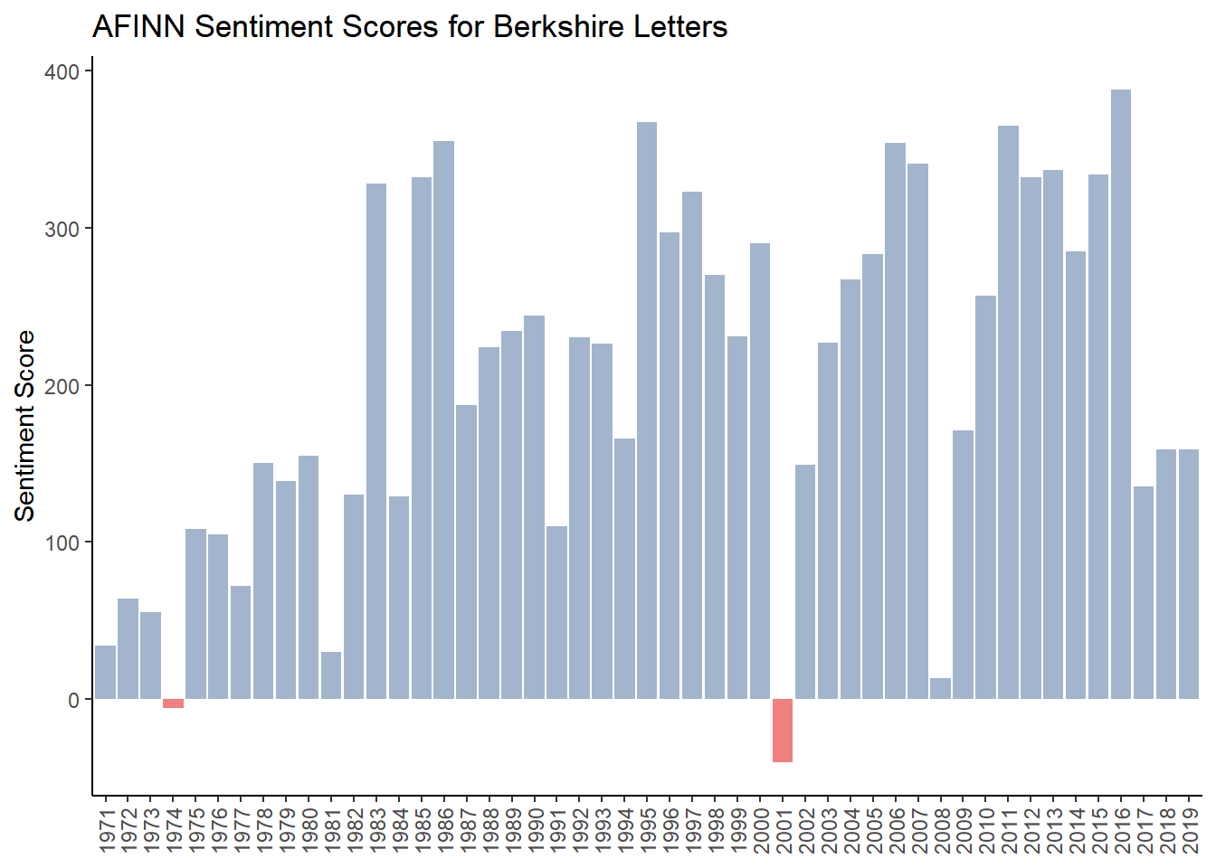
The sentiment using AFINN looks very different than the Bing chart, although “obvious” negative years such as 1974, 2001 and 2008 have either low scores or are negative. With AFINN, 1981 has a low score which makes sense as short term interest rates were 21%, long term rates were 14% as the US was suffering from several years of high inflation. Using the Bing sentiment, 1981 also got a low score.
4.7.2.5 A Brief Glimpse of Performance Data and the Definition of “obvious” Years
In the last paragraph, I used the term “obvious negative years.” I want to briefly explain what that means. Figure 4.4 shows the S&P 500 return over the 49 year period of our analysis. While we will compare sentiment to returns later, I wanted to show returns for the S&P 500 (which is a proxy for the overall performance of the US stock markets) to see which years were negative and where we would expect to see negative sentiment. When I talk about “obvious” periods, they include the 1973-174 bear market, 2000-2002, which includes the dot-com crash and 9/11 and finally, the 2008 financial crisis. These are periods where we would expect more negative sentiment because the markets performed very poorly during these periods.
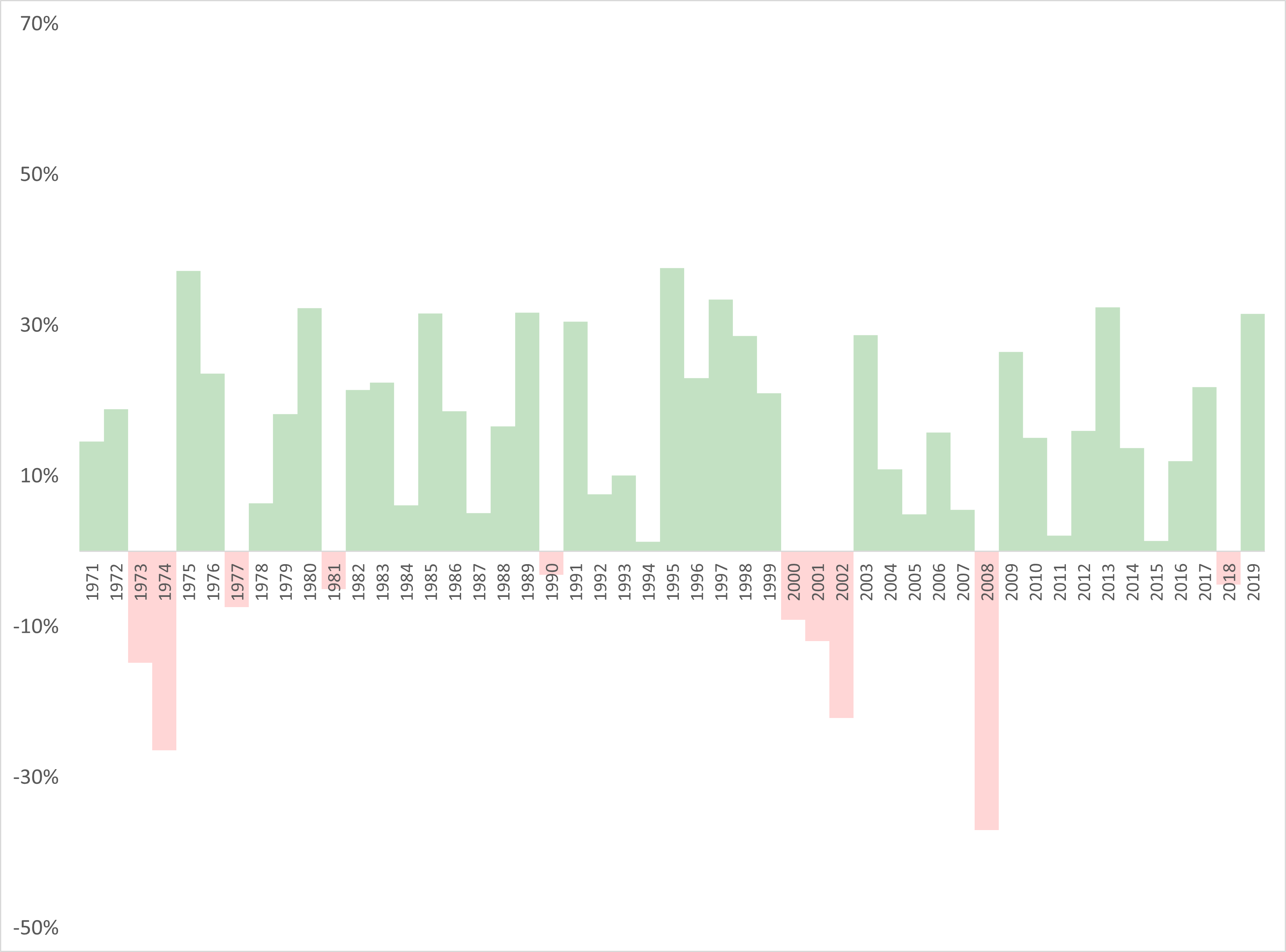
Figure 4.4: S&P 500 Annual Performance
4.7.2.6 A Deeper Look Into How AFINN is Classifying Words
Since the AFINN lexicon scores words from -5 to 5 I decided to multiply the sentiment score for each word by the number of times its used to get a kind of overall impact a given word has using the following code.
brk_afinn %>%
  count(word, sentiment) %>%
#  filter(sentiment ==2) %>%
  mutate(total = sentiment * n) %>%
  arrange(desc(total))
## # A tibble: 1,229 x 4
## word sentiment n total
## <chr> <dbl> <int> <dbl>
## 1 outstanding 5 214 1070
## 2 assets 2 373 746
## 3 worth 2 369 738
## 4 gains 2 367 734
## 5 gain 2 352 704
## 6 shares 1 656 656
## 7 share 1 627 627
## 8 growth 2 272 544
## 9 excellent 3 145 435
## 10 terrific 4 96 384
## # ... with 1,219 more rowsWe see the word “worth” has the second largest impact as it is assigned a positive sentiment of +2. This is problematic as are words like “shares” and “assets” which in context are both likely neutral. This would explain why the average sentiment of the AFINN lexicon is higher than the results we obtained with Bing.
Let’s look at negative words in the same way to see if there are any issues.
brk_afinn %>%
  count(word, sentiment) %>%
  #filter(sentiment <=-4) %>%
  mutate(total = sentiment * n) %>%
  arrange(total)
## # A tibble: 1,229 x 4
## word sentiment n total
## <chr> <dbl> <int> <dbl>
## 1 loss -3 473 -1419
## 2 debt -2 223 -446
## 3 risk -2 200 -400
## 4 bad -3 105 -315
## 5 pay -1 314 -314
## 6 charges -2 130 -260
## 7 casualty -2 121 -242
## 8 catastrophe -3 78 -234
## 9 lost -3 61 -183
## 10 risks -2 91 -182
## # ... with 1,219 more rowsWe see the word “loss” has the greatest influence - since the word can be used in many different contexts with a company that has large insurance operations, it would be suspect. One word that I thought was definitely misclassified is “casualty” which in a generic sense would be negative but in an insurance context would likely be neutral.
4.7.2.7 An Even Deeper Dive into Misclassification of the Word “casualty”
AFINN rates the word “casualty” as a -2, and given that it has 127 mentions, it could have a high influence on the overall sentiment score. Let’s examine which years’ letter uses the word “casualty” the most using this code:
brk_casualty <- brk_afinn %>%
  filter(word == "casualty") %>%   # filters for just the word "worth"
  group_by(year) %>%            # group by year
  count(word, sort = TRUE) %>%  # count total number and sort by frequency
  ungroup()
brk_casualty %>% print(n=5)
## # A tibble: 43 x 3
## year word n
## <chr> <chr> <int>
## 1 1984 casualty 10
## 2 1977 casualty 7
## 3 1986 casualty 7
## 4 1980 casualty 6
## 5 1988 casualty 5
## # ... with 38 more rowsWe see that the 1984 letter has 10 mentions which is the highest. Let’s examine the context where the word “casualty” is used as shown in Figure 4.5.
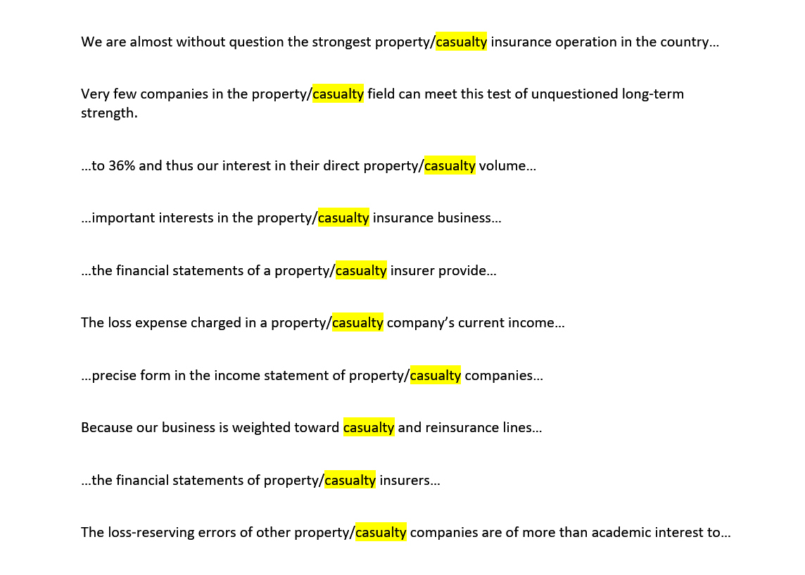
Figure 4.5: Instances of the word casualty in 1984 letter
I was right. The word “casualty” is used 9 out of 10 times as part of the bigram “property/casualty” which is a term specific to the insurance industry. In fact, if you read the first two instances, the sentences are actually extremely positive. To see how are results are skewed for that year, we first look at the overall AFINN score for the 1984 letter which is 129. Since “casualty” is used 10 times and has a value of -2 that implies that the score would be readjusted to 149. And this is just one word in one year’s letter. I am not sure we can rely on these sentiment numbers. But again, the AFINN lexicon has much lower scores for “obvious” years like 1974, 2001 and 2008 so its not completely inaccurate.
Next let’s examine a sentiment lexicon which was expressly designed to analyze financial type documents - the Loughran-McDonald Sentiment Word Lists.
4.7.3 Loughran-McDonald Sentiment Lexicon
4.7.3.1 Description
- Loughran – 2709 words – widely used for in finance for financial statement (10k and 10q) sentiment analysis. Loughran-McDonald Sentiment Word Lists.
4.7.3.2 Combining Loughran with Berkshire Corpus
The following code creates a new dataframe brk_lough and matches words in the Bershire letters with words in the Loughran lexicon.
lough <- get_sentiments(lexicon = "loughran")
brk_lough <- brk_words %>%
  left_join(get_sentiments(lexicon = "loughran"), by = "word") %>%
  mutate(sentiment = ifelse(is.na(sentiment), "neutral", sentiment)) %>%
  group_by(year) %>%
  ungroup()
brk_lough %>% print(n=5)
## # A tibble: 201,855 x 3
## year word sentiment
## <chr> <chr> <chr>
## 1 1971 stockholders neutral
## 2 1971 berkshire neutral
## 3 1971 hathaway neutral
## 4 1971 pleasure positive
## 5 1971 report neutral
## # ... with 201,850 more rowsUnlike the previous lexicons, there are seven different categories. To see unique levels we use the following code:
#to see unique levels
brk_lough %>%
  select(sentiment) %>%
  unique()
## # A tibble: 7 x 1
## sentiment
## <chr>
## 1 neutral
## 2 positive
## 3 negative
## 4 uncertainty
## 5 litigious
## 6 constraining
## 7 superfluous4.7.3.3 Calculating Loughran Sentiment
Since we only want positive and negative sentiment, we will use the following code to calculate a score similar to the way we calculated the sentiment score with the Bing lexicon.
#sentiment by year
brk_lough_year <- brk_lough %>%
  count(year, sentiment) %>%
  spread(key = sentiment, value = n) %>%
  mutate(total = (positive + negative + neutral)) %>%   # create "total" column
  mutate(lough = ((positive - negative) / total)) %>% # create column with calculated score
  select("year", "positive", "negative", "neutral", "total", "lough")  # reorder columns
brk_lough_year %>% print(n=5)
## # A tibble: 49 x 6
## year positive negative neutral total lough
## <chr> <int> <int> <int> <int> <dbl>
## 1 1971 36 22 554 612 0.0229
## 2 1972 41 22 640 703 0.0270
## 3 1973 23 32 778 833 -0.0108
## 4 1974 27 59 628 714 -0.0448
## 5 1975 44 43 853 940 0.00106
## # ... with 44 more rows4.7.3.4 Analysis of Loughran Sentiment
Below is a chart similar to the ones above to analyze the Loughran sentiment results.
g_lough <- ggplot(brk_lough_year, aes(year, lough, fill = lough>0,)) + #fill = makes values below zero in red
  geom_col(show.legend = FALSE) +
  scale_fill_manual(values=c("lightcoral","lightsteelblue3"))+
  labs(x= NULL,y="Sentiment Score",
       title="Loughran Sentiment Scores for Berkshire Letters")+
  theme_classic() +
  theme(axis.text.x = element_text(angle = 90, vjust = 0.5, hjust = 1))
g_lough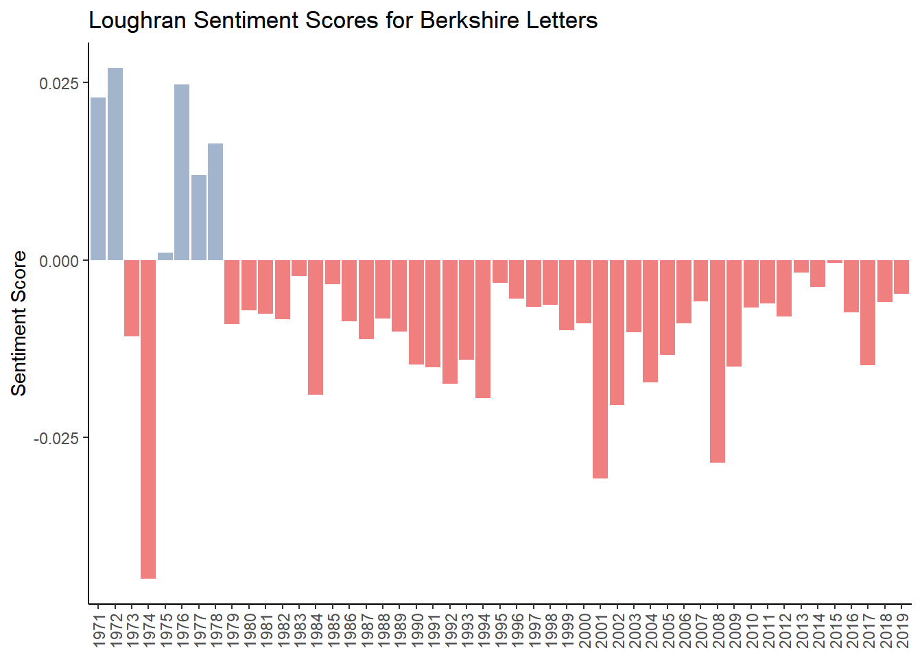
The results look strikingly different. While the “obvious” years of 1974, 2001 and 2008 look in order, the overall sentiment is negative for just about the entire time period. The reason for this might be that of the total of 3,917 words, 2,355 are negative while only 354 are positive. Nevertheless, we will take a closer look at how this lexicon is classifying words to further understand why the scores are so negative.
4.7.3.5 A Deeper Look Into How Loughran is Classifying Words
Let’s do a similar analysis and look at the most frequently used negative words. We see that “loss” and “losses” tops the list as well as “question” and “questions.” I’m not sure why “questions” and “question” would be negative. But we are starting to see a pattern with all three lexicons and the word “loss” and “losses.”
brk_lough %>%
  filter(sentiment == "negative") %>%
  count(word, sentiment, sort = TRUE) %>%
  print(n=5)
## # A tibble: 955 x 3
## word sentiment n
## <chr> <chr> <int>
## 1 loss negative 473
## 2 losses negative 436
## 3 questions negative 141
## 4 question negative 118
## 5 bad negative 105
## # ... with 950 more rowsThe word “loss” appears at the top of the list for all three sentiment lexicons we have used so far. Here is the list again for Bing.
brk_bing %>%
  filter(sentiment == "negative") %>%
  count(word, sentiment, sort = TRUE) %>%
  print(n=3)
## # A tibble: 1,412 x 3
## word sentiment n
## <chr> <chr> <int>
## 1 loss negative 473
## 2 losses negative 436
## 3 debt negative 223
## # ... with 1,409 more rowsFor AFINN “it”loss" is number one but the word “losses” does not show up. Let’s see why.
brk_afinn %>%
  count(word, sentiment) %>%
  #filter(sentiment <=-4) %>%
  mutate(total = sentiment * n) %>%
  arrange(total)%>%
  print(n=3)
## # A tibble: 1,229 x 4
## word sentiment n total
## <chr> <dbl> <int> <dbl>
## 1 loss -3 473 -1419
## 2 debt -2 223 -446
## 3 risk -2 200 -400
## # ... with 1,226 more rowsUsing the code below, we can filter for “losses” in the brk_afinn dataframe. Interestingly, the word does not appear which means that it is not included in the AFINN lexicon.
brk_afinn %>%
  filter(word == "losses")
## # A tibble: 0 x 3
## # ... with 3 variables: year <chr>, word <chr>, sentiment <dbl>4.7.3.6 A Deeper Dive Into the the Classification of the Words “loss” and “losses” in the Three Sentiment Lexicons We Have Looked at So Far.
Let’s do some data wrangling to see which letters use the word “loss” and “losses” the most.
brk_loss_frequency <- brk_words %>%
  filter(word == "losses" | word == "loss") %>%         # filters for words "losses" and "loss"
  count(year, word) %>%                                 # count instances per year
  tidyr::spread(key = word, value = n, fill = 0) %>%    # combines rows and fills nas with 0
  mutate(total = loss + losses) %>%                     # creates new column with total
  arrange(desc(total))                                  # sorts total column in descending order of frequency
brk_loss_frequency %>% print(n=5)
## # A tibble: 49 x 4
## year loss losses total
## <chr> <dbl> <dbl> <dbl>
## 1 2001 24 30 54
## 2 1984 23 17 40
## 3 1990 16 21 37
## 4 2008 18 17 35
## 5 1985 18 16 34
## # ... with 44 more rowsThe years 2001 and 2008 are near the top of the list and are among our “obvious” years. But strangely, 1974 is absent - it shows up at 37 of 49 for frequency of the two words. The 1973-1974 bear market was one of the worst in history. To explore this a bit further, let’s look at the frequency of the use of these two words in chronological order.
brk_loss_frequency$year <- as.numeric(brk_loss_frequency$year) # change "year" column to numeric
g4 <- ggplot(brk_loss_frequency, aes(x = year, y = total)) +
  geom_col(fill = "dodgerblue3", alpha = 0.65) +
   theme_classic() + ylab("Frequency of Words ''loss'' and ''losses'' ")
g4 + theme(axis.title.x = element_blank()) 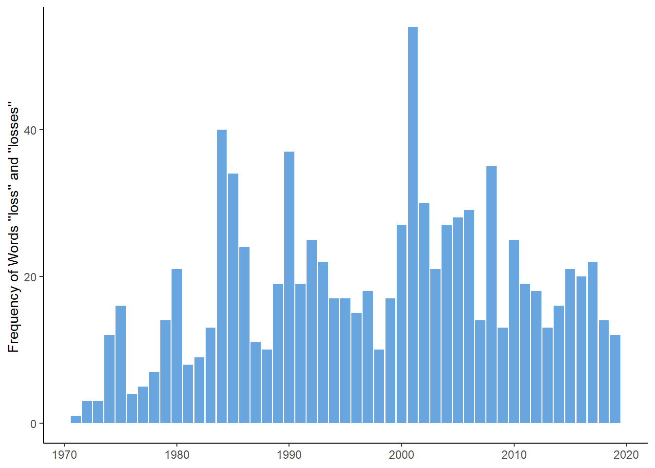
We see a couple of things, the use seems to fluctuate a lot, which could be due to the markets or might be specific to the insurance operations. Also, we are just looking at raw frequency. It might be better to calculate percent of total negative words which I did with the word “worth” previously.
4.7.3.7 Seeing Impact of the Words “loss” and “losses” in the Loughran Lexicon
With the code below, I do some data wrangling, the result of which is a dataframe with the words “loss” and “losses” as percent of negative words and total words for each year in the Loughran lexicon.
#create dataframe with frequency of "loss" and "losses" in descending order
 scrap2 <- brk_lough %>%
  filter(word == "losses" | word == "loss") %>%          # filters for just the word "worth"
  count(year, word) %>%
  tidyr::spread(key = word, value = n, fill = 0) %>%     # combines rows and fills nas with 0
  mutate(total_loss = loss + losses) %>%                 # creates new column with total
  arrange(desc(total_loss))                              # sorts total column in descending order of frequency

#join dataframes and create new columns
brk_loss_lough <- left_join(brk_lough_year, scrap2, by = "year") %>%  # join scrap2 dataframe with brk_lough_year
  mutate(pct_of_neg = (total_loss / negative *100)) %>%               # create new column percent of negative words
  mutate(pct_of_total = (total_loss / total *100)) %>%                # create new column percent of total words
  select("year", "total_loss",  "negative", "pct_of_neg","total", "pct_of_total")

#output of the words "loss" and "losses" as percent of negative words and total words
brk_loss_lough %>%
    select("year", "pct_of_neg", "pct_of_total") %>%
    arrange(desc(pct_of_total)) %>% print(n=5)
## # A tibble: 49 x 3
## year pct_of_neg pct_of_total
## <chr> <dbl> <dbl>
## 1 1975 37.2 1.70
## 2 1974 20.3 1.68
## 3 2001 22.1 1.17
## 4 1984 17.5 0.817
## 5 2008 14.3 0.694
## # ... with 44 more rowsThen to see the frequency of the use of the words and the percent of negative words and total words in a graphical form, I go through the following acrobatics.
# put together new dataframe "scrap3"
scrap3 <- brk_loss_lough %>%
  select("year", "pct_of_neg", "pct_of_total", "total_loss" )

# convert to long form and create new dataframe "scrap3_long"
scrap3_long <- scrap3 %>%
  gather("pct_of_neg", "pct_of_total", "total_loss", key = type, value = percent)

# chart parameters and output
scrap3_long %>%
  ggplot(aes(x = year, y = percent, fill = type)) +
  geom_col() +
  facet_wrap(~ type, ncol = 1, scales = "free_y",
             labeller = as_labeller(c(pct_of_neg = "''Loss'' and ''Losses'' as % of Negative Words ",
                                        pct_of_total = "''Loss'' and ''Losses'' as % of Total Words",
                                        total_loss = "Frequency of words ''Loss'' and ''Losses''"))) +
  theme_bw() +
  theme(legend.position = "none") +
  xlab(NULL) + ylab(NULL) +
theme(axis.text.x=element_text(angle=90, vjust=.5, hjust=0),panel.grid = element_blank()) 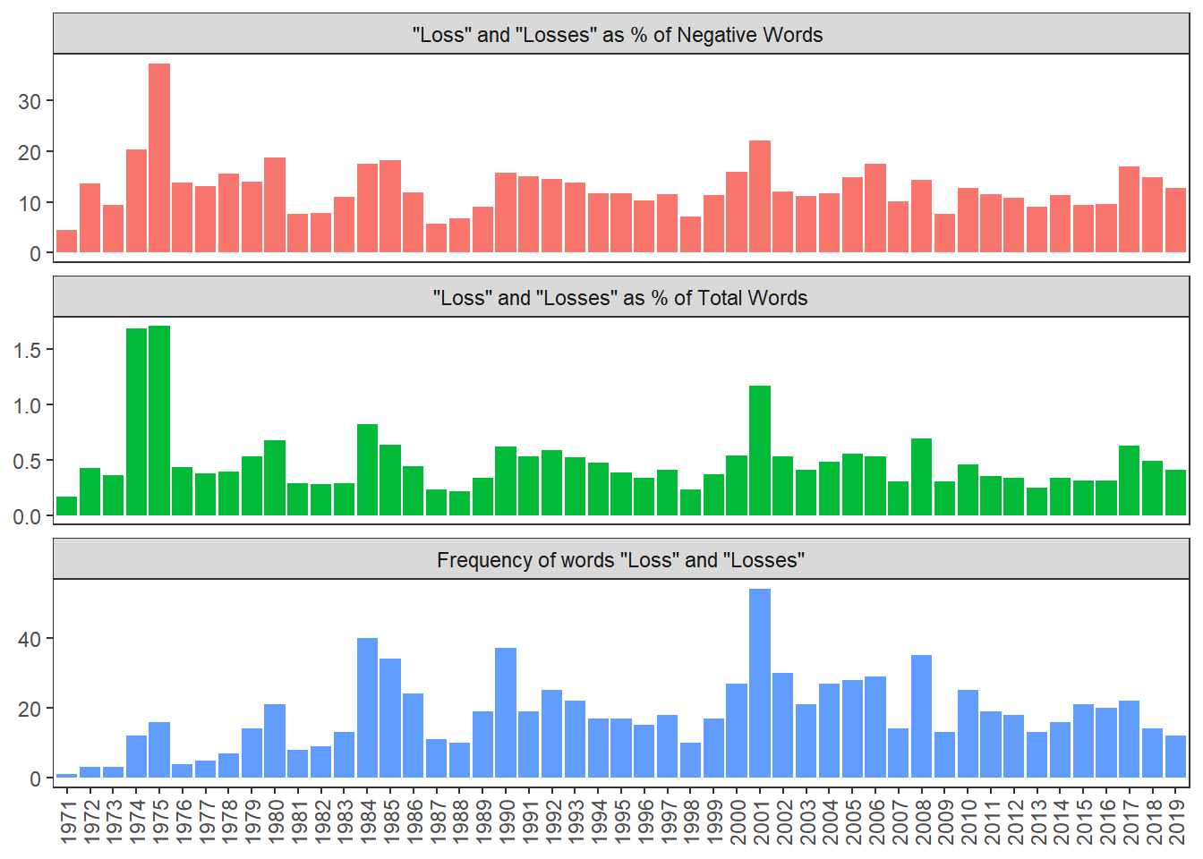
What we see is that “loss” and “losses” accounts for a very high percent of negative words in 1974 (20%) and 1975(37%). But it is surprising that the overall Loughran score is positive for 1975. While “losses” and “loss” are used the most in the 2001 letter, it is 22% of all the negative words used in that year.
We can see this on the following table, since the 1974 and 1975 letters are so much shorter, the lower frequency has more of an impact than on the 2001 letter.
brk_loss_lough %>%
  filter(year == "1974" | year == "1975" | year == "2001")
## # A tibble: 3 x 6
## year total_loss negative pct_of_neg total pct_of_total
## <chr> <dbl> <int> <dbl> <int> <dbl>
## 1 1974 12 59 20.3 714 1.68
## 2 1975 16 43 37.2 940 1.70
## 3 2001 54 244 22.1 4622 1.17Over the entire time period, “loss” and “losses” as a percent of negative words are 12.9%. It strikes me as odd that the word “loss” and “losses” would be used so much in a negative context in Berkshire’s letters. The words are probably being used in conjunction with the insurance operations in a neutral context. But that’s just a guess. At this point, we have to see how these words are used in context to determine if they are misclassified.
I think it would be interesting to look more into the 1975 letter because the word “loss” and “losses” is used a lot but the overall sentiment for the year is positive. As shown in the table below where the last column has the overall sentiment for that year. While loss is used 16 times in 1975 and comprises 37% of the negative words, the overall year is positive - strange…
brk_loss_lough %>%
  select("year", "total_loss", "pct_of_neg") %>%                      # selects certain columns to join
  left_join(brk_lough_year, brk_loss_lough,  by = "year") %>%         # joins the two dataframes
  filter(year == "1974" | year == "1975" | year == "2001") %>%        # selects certain years
  select("year", "total_loss", "negative", "pct_of_neg",
         "total", "lough")                                            # reorders columns
## # A tibble: 3 x 6
## year total_loss negative pct_of_neg total lough
## <chr> <dbl> <int> <dbl> <int> <dbl>
## 1 1974 12 59 20.3 714 -0.0448
## 2 1975 16 43 37.2 940 0.00106
## 3 2001 54 244 22.1 4622 -0.0307Reading through the 1975 letter, it appears that of the 16 instances, a portion are in the context of losses in prior years, a portion are losses in the businesses in the current year and a number of instances relate to the insurance operations - in one case it talked about the company having the “lowest loss ratio” which is actually positive, or the bank operations where the term “net loan losses” is an industry term and not necessarily negative. Here again, looking at bigrams or trigrams such as “loss ratio” or “net loan losses” and classifiying them separate from “loss” and “losses” might improve the accuracy of the sentiment analysis. This also might explain why the Loughran lexicon shows Berkshire having consistent negative sentiment - it could be due to terms that in context would be classified as neutral.
Incidentally, I went back to look at how the Loughran lexicon treats the word “casualty” which we saw was misclassified by the other lexicons. It classified it as neutral which in the case of Berkshire, is correct. I talk about this a little more in the notes in Chapter 10.
4.7.3.8 Final Thoughts on Loughran Lexicon
While it was concerning that sentiment appeared to be negative in most of the time periods - in contrast to Bing and AFINN - as long as the apparent misclassifications are consistent over time, they won’t prove to be a problem. We will keep this in mind as we go through the remaining lexicons.
4.7.4 NRC Sentiment Lexicon
4.7.4.1 Description
NRC: The NRC Emotion Lexicon is a list of 5,636 English words and their associations with eight basic emotions (anger, fear, anticipation, trust, surprise, sadness, joy, and disgust) and two sentiments (negative and positive). The annotations were manually done by crowdsourcing on Amazon Mechanical Turk and detailed in a paper by Mohammad and Turney (2013). The unique levels are revealed using the following code.
#to see unique levels
tidytext::get_sentiments("nrc")  %>%
  select(sentiment) %>%
  unique()
## # A tibble: 10 x 1
## sentiment
## <chr>
## 1 trust
## 2 fear
## 3 negative
## 4 sadness
## 5 anger
## 6 surprise
## 7 positive
## 8 disgust
## 9 joy
## 10 anticipation4.7.4.2 Combining NRC with Berkshire Corpus
Next we filter the dataframe for just sentiment and then create a new dataframe brk_nrc and match it with the words in the Berkshire letters.
# create dataframe with just NRC sentiment
nrc <- get_sentiments("nrc") %>%
  filter(sentiment == "negative" | sentiment == "positive") #filter for just sentiment

# join NRC with "brk_words"
brk_nrc <- brk_words %>%
  left_join(nrc, by = "word") %>%
  mutate(sentiment = ifelse(is.na(sentiment), "neutral", sentiment)) %>%
  group_by(year) %>%
  ungroup()
brk_nrc %>% print(n=5)
## # A tibble: 202,647 x 3
## year word sentiment
## <chr> <chr> <chr>
## 1 1971 stockholders neutral
## 2 1971 berkshire neutral
## 3 1971 hathaway neutral
## 4 1971 pleasure neutral
## 5 1971 report neutral
## # ... with 202,642 more rows4.7.4.3 Calculating NRC Sentiment
Then we use the following code to calculate sentiment in the same way that we calculated Bing and Loughran sentiment and aggregate by year to get a sentiment score for each year.
#sentiment by year
brk_nrc_year <- brk_nrc %>%
  count(year, sentiment) %>%
  spread(key = sentiment, value = n) %>%
  mutate(total = (positive + negative + neutral)) %>%   # create "total" column
  mutate(nrc = ((positive - negative) / total)) %>% # create column with calculated score
  select("year", "positive", "negative", "neutral", "total", "nrc")  # reorder columns
brk_nrc_year %>% print(n=5)
## # A tibble: 49 x 6
## year positive negative neutral total nrc
## <chr> <int> <int> <int> <int> <dbl>
## 1 1971 80 27 513 620 0.0855
## 2 1972 107 32 586 725 0.103
## 3 1973 107 44 709 860 0.0733
## 4 1974 83 60 594 737 0.0312
## 5 1975 159 57 758 974 0.105
## # ... with 44 more rowsWe have achieved what we set out to do - create a dataframe brk_nrc_year with a column for year and a second column of with the NRC sentiment score.
4.7.4.4 Analysis of NRC Sentiment
We can now chart the sentiment scores for each year which is shown below. We see that the NRC lexcion scores sentiment consitently higher than zero which must mean it is classifying words differently than the other lexicons. But our “obvious” years - 1974, 2001 and 2008 are noticably lower.
g5 <- ggplot(brk_nrc_year, aes(year, nrc)) +
  geom_col(show.legend = FALSE, fill = "lightsteelblue3") +
  labs(x= NULL,y=NULL,
       title="NRC Sentiment Scores for Berkshire Letters")+
  theme_classic() +
  theme(axis.text.x = element_text(angle = 90, vjust = 0.5, hjust = 1))
g5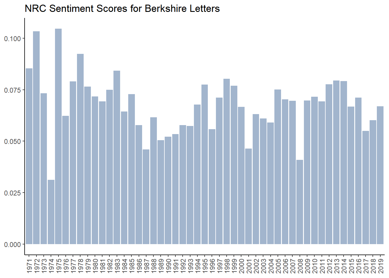
4.7.4.5 A Deeper Look Into How NRC is Classifying Words
If we look at word frequency of positive words, we see the top 10 list populated with words classified as positive which should be classified as neutral like “share,” “money,” “worth,” “equity” and “management.” That explains why the sentiment is so consistently high.
brk_nrc %>%
  filter(sentiment == "positive") %>%
  count(word, sentiment, sort = TRUE)
## # A tibble: 1,236 x 3
## word sentiment n
## <chr> <chr> <int>
## 1 share positive 627
## 2 major positive 618
## 3 money positive 490
## 4 income positive 488
## 5 cash positive 416
## 6 assets positive 373
## 7 worth positive 369
## 8 equity positive 364
## 9 gain positive 352
## 10 management positive 352
## # ... with 1,226 more rowsWhen I looked at frequency I saw words classified as negative that in the context of Berkshire, wouldn’t be negative such as “tax,” “bonds,” “stocks,” “debt” and “casualty.” But then I noticed that “outstanding” is classified as negative as is “income.”
brk_nrc %>%
  filter(sentiment == "negative") %>%
  count(word, sentiment, sort = TRUE)
## # A tibble: 1,209 x 3
## word sentiment n
## <chr> <chr> <int>
## 1 tax negative 748
## 2 income negative 488
## 3 loss negative 473
## 4 bonds negative 303
## 5 stocks negative 266
## 6 debt negative 223
## 7 outstanding negative 214
## 8 risk negative 200
## 9 expenses negative 157
## 10 inflation negative 125
## # ... with 1,199 more rowsIt seemed odd to me that “income” showed up on both positive and negative lists and “outstanding” showed up as negative. I thought there might have been an error with how I collected or coded the data but I couldn’t find any problems. When I filter the NRC lexicon for the words “income” and “outstanding” they show up on both lists.
nrc %>%
  filter(word == "outstanding" | word == "income") %>%
  count(word, sentiment, sort = TRUE)
## # A tibble: 4 x 3
## word sentiment n
## <chr> <chr> <int>
## 1 income negative 1
## 2 income positive 1
## 3 outstanding negative 1
## 4 outstanding positive 1I emailed the author of the lexicon but have yet to hear back. Chances are it is my mistake13.
4.7.5 Syuzhet Sentiment Lexicon
4.7.5.1 Description
The Syuzhet lexicon is part of the Syuzhet package developed by Matthew Jockers. The lexicon was developed in the Nebraska Literary Lab and contains 10,748 words which are assigned a score of -1 to 1 with 16 gradients (Jockers and Thalken 2020). As seen in the descriptive statistics below, the mean is -0.213.
syuzhet <- get_sentiment_dictionary("syuzhet") #get lexicon and create dataframe
#descriptive statistics
summary(syuzhet)
## word value
## Length:10748 Min. :-1.000
## Class :character 1st Qu.:-0.750
## Mode :character Median :-0.400
## Mean :-0.213
## 3rd Qu.: 0.400
## Max. : 1.0004.7.5.2 Combining Syuzhet Lexicon with Berkshire Corpus
Since the Syuzhet lexcion does not contain any neutral words we can use the inner_join command which automatically filters out words in the brk_words dataframe which are not found in the Syuzhet lexicon.
brk_syuzhet <- brk_words %>%      #creates new dataframe "brk_syuzhet"
  inner_join(syuzhet, by = "word") #just joins words in syuzhet
brk_syuzhet
## # A tibble: 47,205 x 3
## year word value
## <chr> <chr> <dbl>
## 1 1971 pleasure 0.5
## 2 1971 excluding -0.8
## 3 1971 gains 0.5
## 4 1971 equity 1
## 5 1971 inadequate -0.75
## 6 1971 benefits 1
## 7 1971 continue 0.4
## 8 1971 objective 0.4
## 9 1971 management 0.4
## 10 1971 improve 0.75
## # ... with 47,195 more rows4.7.5.3 Calculating syuzhet sentiment by year
As you can see from the previous table, Syuzhet assigns each word a sentiment score from -1 to +1. In order to produce a sentiment score by year, we simply sum up all the values for a particular year using the following code:
#sentiment by year
brk_syuzhet_year <- brk_syuzhet %>%
  group_by(year) %>%
  summarise(syuzhet = sum(value)) %>%
  ungroup()
brk_syuzhet_year %>% print(n=5)
## # A tibble: 49 x 2
## year syuzhet
## <chr> <dbl>
## 1 1971 36.0
## 2 1972 56.6
## 3 1973 43.8
## 4 1974 8.6
## 5 1975 69.2
## # ... with 44 more rows4.7.5.4 Analyis of syuzhet sentiment
The following chart shows Syuzhet sentiment score for each of the 49 letters. The sentiment is positive throughout the entire period which is a bit odd because of the 10,748 total words, 7,161 are negative and 3,587 are positive. But it is encouraging that our “obvious” years of 1974, 2001 and 2008 are the lowest. A deeper dive needs to be done to investigate why scores are so positive.
g_syuzhet <- ggplot(brk_syuzhet_year, aes(year, syuzhet)) +
  geom_col(show.legend = FALSE, fill = "lightsteelblue3") +
  labs(x= NULL,y="Sentiment Score",
       title="Syuzhet Sentiment Scores for Berkshire Letters")+
  theme_classic() +
  theme(axis.text.x = element_text(angle = 90, vjust = 0.5, hjust = 1))
g_syuzhet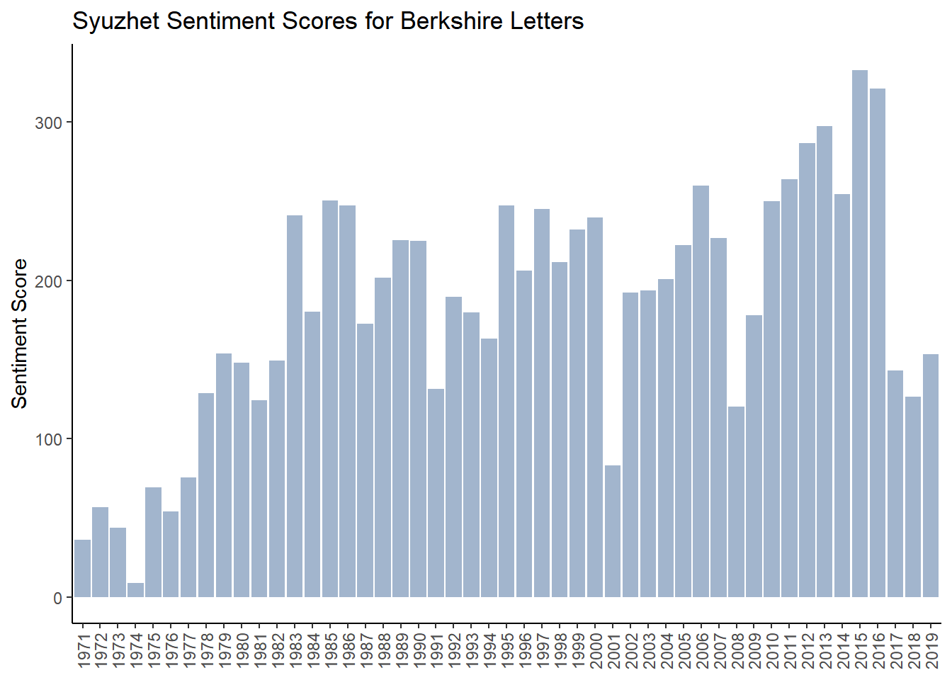
4.7.5.5 A Deeper Look Into How Syuzhet is Classifying Words
Since the Syuzhet lexicon scores words from -1 to 1 I decided to multiply the sentiment score for each word by the number of times its used to get a kind of overall impact a given word has using the following code (exactly what I did with the AFINN lexicon). Words that are used frequently and / or have high positivity scores result in high impact.
In my opinion, most of the words in the top 10 list below should be classified as neutral rather than positive. This would explain why the sentiment scores are consistently high.
brk_syuzhet %>%
  count(word, value) %>%
  mutate(impact = value * n) %>%
  arrange(desc(impact))
## # A tibble: 3,904 x 4
## word value n impact
## <chr> <dbl> <int> <dbl>
## 1 equity 1 364 364
## 2 share 0.5 627 314.
## 3 money 0.6 490 294
## 4 worth 0.75 369 277.
## 5 gain 0.75 352 264
## 6 major 0.4 618 247.
## 7 assets 0.5 373 186.
## 8 gains 0.5 367 184.
## 9 cash 0.4 416 166.
## 10 ownership 0.6 268 161.
## # ... with 3,894 more rowsWhen we examine negative words sorted by impact we see some of the same words that were problematic in the other lexicons - “loss,” “losses” and “casualty.” There are other words which have a sizable impact such as “tax” and “debt” which in Berkshire’s case should likely be categorized as neutral.
brk_syuzhet %>%
  count(word, value) %>%
  mutate(impact = value * n) %>%
  arrange(impact)
## # A tibble: 3,904 x 4
## word value n impact
## <chr> <dbl> <int> <dbl>
## 1 loss -0.75 473 -355.
## 2 losses -0.8 436 -349.
## 3 tax -0.25 748 -187
## 4 debt -0.75 223 -167.
## 5 risk -0.75 200 -150
## 6 casualty -0.75 121 -90.8
## 7 economic -0.25 339 -84.8
## 8 bad -0.75 105 -78.8
## 9 inflation -0.6 125 -75
## 10 liability -0.5 131 -65.5
## # ... with 3,894 more rows4.7.5.6 Final Words on Syuzhet Lexicon
This lexicon is presenting the same issues as the previous lexicons in analyzing the Berkshire letters. Since it wasn’t designed for analyzing financial and business texts, we can hardly make any criticisms.
4.7.6 SenticNet4 Sentiment Lexicon
The SenticNet and Sentiword lexicons are both accessed through the lexicon package in R developed by Tyler Rinker (2018)
4.7.6.1 Description
SenticNet was developed at the MIT Media Laboratory in 2009. It replaces bag-of-words models “…with a new model that sees text as a bag of concepts and narratives” (SenticNet n.d.). It contains 23,626 words (11,774 positive and 11,852 negative) scored on a continuous scale between -1 and 1. The mean is -0.062.
While the authors of the lexicon say that SenticNet can be used like any other lexicon, they acknowledge that the “right way” to use it is for task of polarity detection in conjunction with sentic patterns(Cambria et al. 2016). As I don’t understand what “polarity detection” or “sentic patterns” are yet, I will use it like any other lexicon.
#create dataframe with lexicon
senticnet <- hash_sentiment_senticnet
#rename columns
senticnet <- senticnet %>% rename(word = x, value = y)
#descriptive statistics
summary(senticnet)
## word value
## Length:23626 Min. :-0.98000
## Class :character 1st Qu.:-0.63000
## Mode :character Median :-0.02000
## Mean :-0.06175
## 3rd Qu.: 0.55900
## Max. : 0.98200Using the code below, we match up the words that are in the SenticNet lexicon with the corresponding words in the Berkshire letters. Using the inner_join command automatically filters out words in the brk_words dataframe which are not found in the SenticNet lexicon
4.7.6.2 Combining Senticnet Sentiment Lexicon With Berkshire Corpus
brk_senticnet <- brk_words %>%
  inner_join(senticnet, by = "word")

brk_senticnet
## # A tibble: 114,305 x 3
## year word value
## <chr> <chr> <dbl>
## 1 1971 pleasure 0.531
## 2 1971 report -0.51
## 3 1971 earnings 0.828
## 4 1971 capital 0.067
## 5 1971 beginning -0.8
## 6 1971 equity 0.037
## 7 1971 result 0.044
## 8 1971 average 0.071
## 9 1971 american 0.097
## 10 1971 industry 0.123
## # ... with 114,295 more rows4.7.6.3 Calculating SenticNet Sentiment
#sentiment by year
brk_senticnet_year <- brk_senticnet  %>%
  group_by(year) %>%
  summarise(senticnet  = sum(value)) %>%
  ungroup()
brk_senticnet_year %>% print(n=5)
## # A tibble: 49 x 2
## year senticnet
## <chr> <dbl>
## 1 1971 60.1
## 2 1972 76.7
## 3 1973 60.5
## 4 1974 33.2
## 5 1975 89.9
## # ... with 44 more rows4.7.6.4 Analysis of SenticNet Sentiment
g_senticnet  <- ggplot(brk_senticnet_year, aes(year, senticnet)) +
  geom_col(show.legend = FALSE , fill = "lightsteelblue3") +
  labs(x= NULL,y="Sentiment Score",
       title="Senticnet Sentiment Scores for Berkshire Letters")+
  theme_classic() +
  theme(axis.text.x = element_text(angle = 90, vjust = 0.5, hjust = 1))
g_senticnet 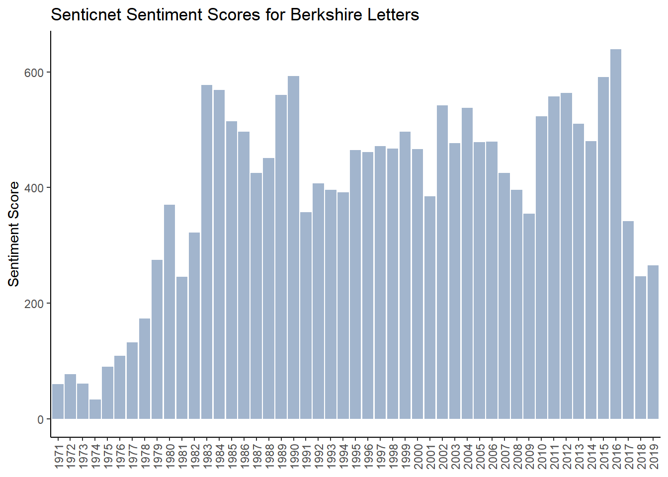
4.7.6.5 A Deeper Look Into How SenticNet is Classifying Words
4.7.7 Sentiword Sentiment Lexicon
4.7.7.1 Description
Sentiword was developed at the MIT Media Laboratory in 2009. It replaces bag-of-words models “…with a new model that sees text as a bag of concepts and narratives” (SenticNet n.d.). It as developed to try and blend manually built and automatically derived lexicon classification methods (Baccianella, Esuli, and Sebastiani 2010), (Gatti, Guerini, and Turchi 2016). It contains 23,626 words (11,774 positive and 11,852 negative) scored on a continuous scale between -1 and 1. The mean is -0.062.
#create dataframe with lexicon
sentiword  <- hash_sentiment_sentiword
#rename columns
sentiword <- sentiword %>% rename(word = x, value = y)
#descriptive statistics
summary(sentiword)
## word value
## Length:20093 Min. :-1.00000
## Class :character 1st Qu.:-0.25000
## Mode :character Median :-0.12500
## Mean :-0.06174
## 3rd Qu.: 0.25000
## Max. : 1.000004.7.7.2 Combining Sentiword Sentiment Lexicon With Berkshire Corpus
Using the code below, we match up the words that are in the Sentiword lexicon with the corresponding words in the Berkshire letters. Using the inner_join command automatically filters out words in the brk_words dataframe which are not found in the Sentiword lexicon
brk_sentiword <- brk_words %>%
  inner_join(sentiword, by = "word")

brk_sentiword
## # A tibble: 46,269 x 3
## year word value
## <chr> <chr> <dbl>
## 1 1971 pleasure 0.312
## 2 1971 beginning 0.125
## 3 1971 result 0.25
## 4 1971 average -0.375
## 5 1971 inadequate -0.562
## 6 1971 improve 0.375
## 7 1971 return 0.0938
## 8 1971 capitalization 0.125
## 9 1971 return 0.0938
## 10 1971 rate -0.125
## # ... with 46,259 more rows4.7.7.3 Calculating Sentiword Sentiment
#sentiment by year
brk_sentiword_year <- brk_sentiword  %>%
  group_by(year) %>%
  summarise(sentiword  = sum(value)) %>%
  ungroup()
brk_sentiword_year
## # A tibble: 49 x 2
## year sentiword
## <chr> <dbl>
## 1 1971 14.7
## 2 1972 20.8
## 3 1973 -1.61
## 4 1974 -2.54
## 5 1975 28.0
## 6 1976 25.7
## 7 1977 22.5
## 8 1978 15.8
## 9 1979 20.8
## 10 1980 39.0
## # ... with 39 more rows4.7.7.4 Analysis of Sentiword Sentiment
g_sentiword  <- ggplot(brk_sentiword_year, aes(year, sentiword , fill = sentiword >0,)) + #fill = makes values below zero in red
  geom_col(show.legend = FALSE) +
  scale_fill_manual(values=c("lightcoral","lightsteelblue3"))+
  labs(x= NULL,y="Sentiment Score",
       title="Sentiword Sentiment Scores for Berkshire Letters")+
  theme_classic() +
  theme(axis.text.x = element_text(angle = 90, vjust = 0.5, hjust = 1))
g_sentiword 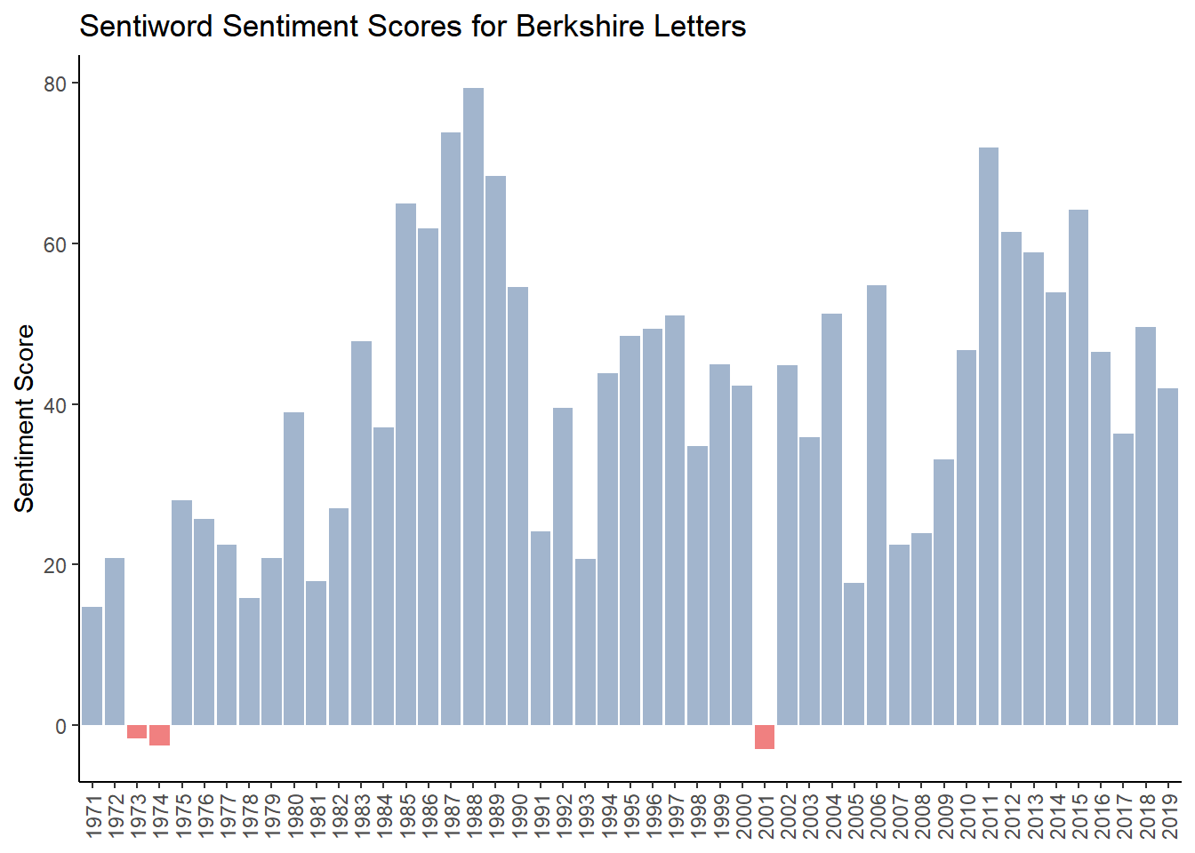
4.7.7.5 A Deeper Look Into How Sentiword is Classifying Words
4.7.8 SO-CAL Lexicon
4.7.8.1 Description
SO-CAL (Semantic Orientation CALculator) began development in 2004. Words in the lexicon are annotated with their semantic orientation or polarity. The calculation of sentiment in SOCAL rests on two assumptions: that individual words have polarity independent of context and that this semaintic orientation can be expressed as a numerical value. The lexicon was classified with Amazon Mechanical Turk (Taboada et al. 2011).
SO-CAL is written in Python and since I am still a Python novice, I decided to download the text files from GitHub and do the analysis in R. I downloaded several dictionaries (adjectives, adverbs, nouns, verbs and and combined them together. Since a small number of words appear in multiple dictionaries, I simply took the average score. The dataframe I created contains 5,971 words (2,438 positive and 3,530 negative) scored on a continuous scale between -5 and 5. The mean is -0.34.
#Import SOCAL lexicon to dataframe
socal<- read_csv("C:\\Users\\psonk\\Dropbox\\111 TC\\R stuff\\NLP\\berkshire\\socal_mean.csv",
                  col_names = FALSE)
#Data Wrangling
socal <- socal %>% rename(word = X1, value = X2)
socal <- socal[-c(1),]
socal$value <- as.numeric(socal$value)

summary(socal)
## word value
## Length:5971 Min. :-5.0000
## Class :character 1st Qu.:-2.0000
## Mode :character Median :-1.0000
## Mean :-0.3406
## 3rd Qu.: 2.0000
## Max. : 5.00004.7.8.2 Combining SOCAL Sentiment Lexicon With Berkshire Corpus
Using the code below, we match up the words that are in the SOCAL lexicon with the corresponding words in the Berkshire letters. Using the inner_join command automatically filters out words in the brk_words dataframe which are not found in the SOCAL lexicon.
brk_socal <- brk_words %>%
  inner_join(socal, by = "word")

brk_socal %>% print(n=5)
## # A tibble: 28,313 x 3
## year word value
## <chr> <chr> <dbl>
## 1 1971 pleasure 3
## 2 1971 average 1
## 3 1971 inadequate -2
## 4 1971 improve 2
## 5 1971 difficult -2
## # ... with 28,308 more rows4.7.8.3 Calculating SOCAL Sentiment by Year
#sentiment by year
brk_socal_year <- brk_socal  %>%
  group_by(year) %>%
  summarise(socal  = sum(value)) %>%
  ungroup()
brk_socal_year %>% print(n=5)
## # A tibble: 49 x 2
## year socal
## <chr> <dbl>
## 1 1971 63.5
## 2 1972 118.
## 3 1973 102.
## 4 1974 17.5
## 5 1975 136.
## # ... with 44 more rows4.7.8.4 Analysis of SOCAL Sentiment
g_socal <- ggplot(brk_socal_year, aes(year, socal , fill = socal >0,)) + #fill = makes values below zero in red
geom_col(show.legend = FALSE) +
scale_fill_manual(values=c("lightsteelblue3","lightcoral"))+
labs(x= NULL,y="Sentiment Score",
title="SOCAL Sentiment Scores for Berkshire Letters")+
theme_classic() +
theme(axis.text.x = element_text(angle = 90, vjust = 0.5, hjust = 1))
g_socal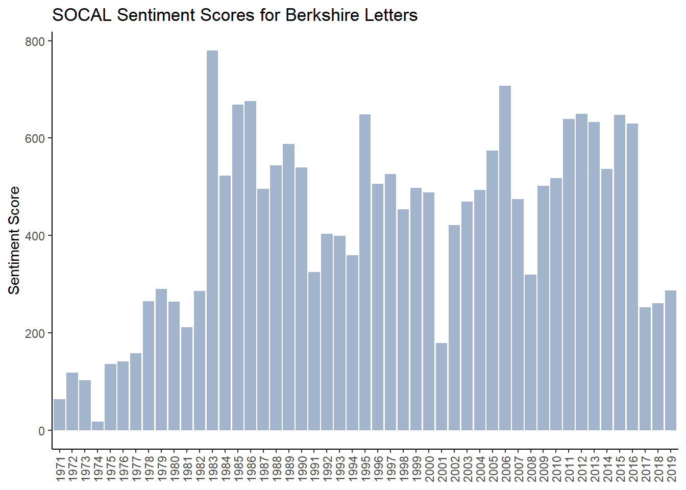 #### A Deeper Look Into How SOCAL is Classifying Words
We see that SOCAL has some of the same issues the other lexica have with positive words such as “economic,” “share” and “worth” which are all in our top ten list in term of impact.
brk_socal %>%
  count(word, value) %>%
  mutate(impact = value * n) %>%
  arrange(desc(impact))
## # A tibble: 2,289 x 4
## word value n impact
## <chr> <dbl> <int> <dbl>
## 1 outstanding 5 214 1070
## 2 economic 3 339 1017
## 3 profit 2 442 884
## 4 excellent 5 145 725
## 5 gain 2 352 704
## 6 extraordinary 5 138 690
## 7 share 1 627 627
## 8 worth 1.67 369 615.
## 9 special 3 194 582
## 10 terrific 5 96 480
## # ... with 2,279 more rowsAnd it also has the same issues with negative words such as “loss,” “catastrophe” and “casualty.”
brk_socal %>%
  count(word, value) %>%
  mutate(impact = value * n) %>%
  arrange(impact)
## # A tibble: 2,289 x 4
## word value n impact
## <chr> <dbl> <int> <dbl>
## 1 loss -2 473 -946
## 2 cost -1 718 -718
## 3 liability -3 131 -393
## 4 catastrophe -5 78 -390
## 5 bad -3 105 -315
## 6 expense -2 132 -264
## 7 casualty -2 121 -242
## 8 terrible -5 46 -230
## 9 worse -4 54 -216
## 10 difficult -2 103 -206
## # ... with 2,279 more rowsExamining the word “outstanding.”
brk_words %>%
  count(year, word) %>%
  filter(word == "outstanding") %>%
  group_by(year) %>%
  arrange(desc(n)) %>%
  ungroup() %>% print(n=5)
## # A tibble: 47 x 3
## year word n
## <chr> <chr> <int>
## 1 1995 outstanding 9
## 2 1996 outstanding 9
## 3 2000 outstanding 9
## 4 2006 outstanding 9
## 5 2012 outstanding 9
## # ... with 42 more rows4.8 Correlation of Sentiment Measures
Because several of the lexica are on different scales, in order to analyze them, I computed z-scores for each. I’ll show a before and after with the AFINN lexicon as an example. Here is the “before” graph of AFINN sentiment.
Next is to calculate the z-scores, which is the individual observation minus the mean divided by standard deviation \(z = \frac{x- \mu}{\sigma}\). Using this code below, we see our output has two columns, one with the raw score and another with the z-score.
brk_afinn_year %>%
  mutate(afinn_z = ((brk_afinn_year$afinn - mean(brk_afinn_year$afinn))/ sd(brk_afinn_year$afinn))) %>%
  select(year, afinn, afinn_z)
## # A tibble: 49 x 3
## year afinn afinn_z
## <chr> <dbl> <dbl>
## 1 1971 34 -1.52
## 2 1972 64 -1.26
## 3 1973 55 -1.34
## 4 1974 -6 -1.87
## 5 1975 108 -0.867
## 6 1976 105 -0.893
## 7 1977 72 -1.18
## 8 1978 150 -0.495
## 9 1979 139 -0.593
## 10 1980 155 -0.451
## # ... with 39 more rowsThe graphed “after” output looks very different.
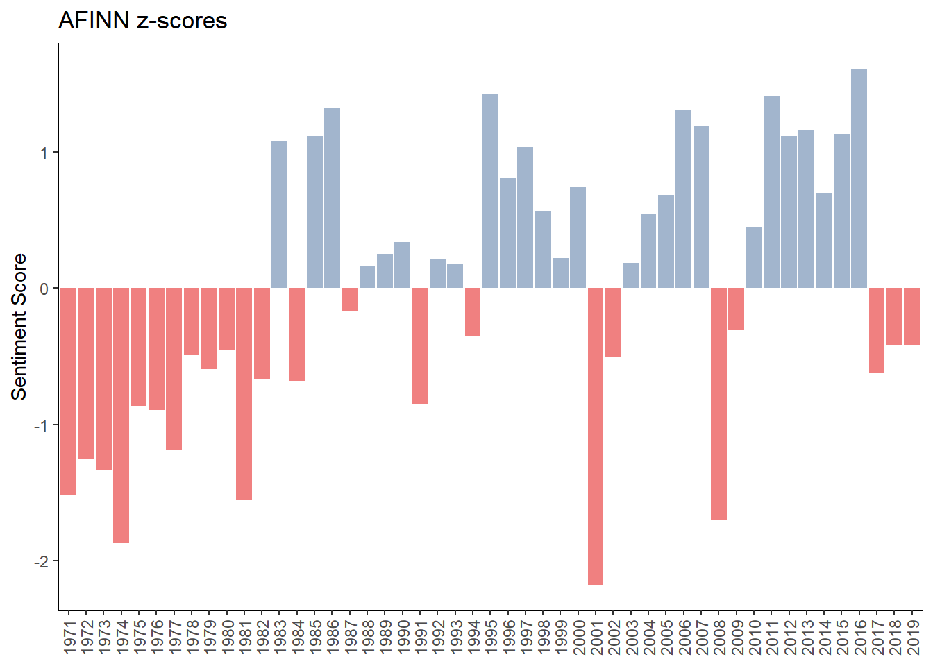
Repeating this z-score calculation for all the lexicons results in the graph below.
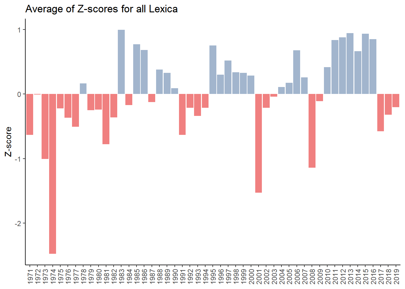
Our “obvious” negative years - 1974, 2001 and 2008 are the most negative. Looking back to Figure 4.4 which is shown again below we see there is some correlation between sentiment and the performance of the S&P 500. But again, this is just foreshadowing, we will go more in-depth into performance and sentiment in Chapter 5.
Figure 4.6: S&P 500 Annual Performance
4.8.1 Correlation Analysis of Sentiment Lexica
4.8.1.1 Correlation Matrix
The matrix in Figure 4.7 shows the the correlations of the various lexicons.
# rename so it looks prettier
brk_all_sentiment <- brk_all_sentiment  %>% rename(afinn = afinn_z, bing = bing_z, socal = socal_z, lough = lough_z, syuzhet = syuzhet_z, senticnet = senticnet_z, sentiword = sentiword_z, nrc = nrc_z)

# ggpairs correlation matrix
corr_for_ggpairs <- ggpairs(brk_all_sentiment, columns = c("afinn", "bing", "socal", "lough", "syuzhet", "senticnet", "sentiword", "nrc", "mean"))

# ggpairs correlation matrix in hi-res
ggsave(corr_for_ggpairs, filename = "corr_for_ggpairs.png", dpi = 300, type = "cairo",
       width = 8, height = 6, units = "in")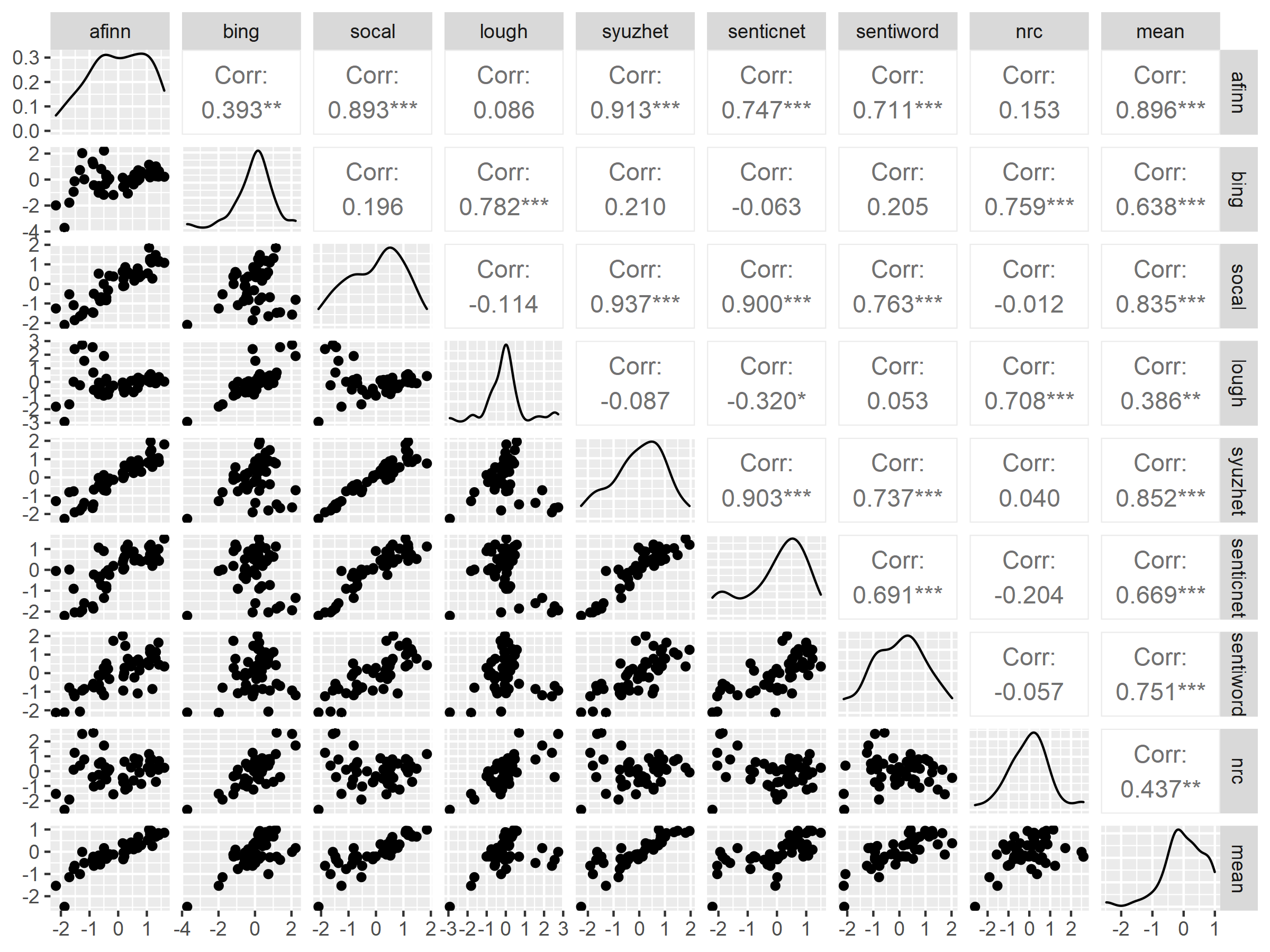
Figure 4.7: Correlation of Sentiment Dictionaries
I decided to also display the results in a more graphical way and using the corrplot package which helps identify hidden structure and patterns in the matrix. While one could eyeball the matrix and see that certain lexicons are less correlated with others, using hierarchical clustering order in the corrplot package really makes this relationship jump out.
# dataframe for correlation matrix
m <- brk_all_sentiment %>%
select(-c(year))
#correlation matrix
corr_matrix <- cor(m)
#as_tibble(corr_matrix)
#nicer colors
col<- colorRampPalette(c("red", "white", "royalblue"))(20)
#correlation matrix with h clustering
corrplot::corrplot(corr_matrix, method = "number", order = "hclust", addrect = 2, tl.col = "black", tl.srt = 45, col = col, number.cex=.85 )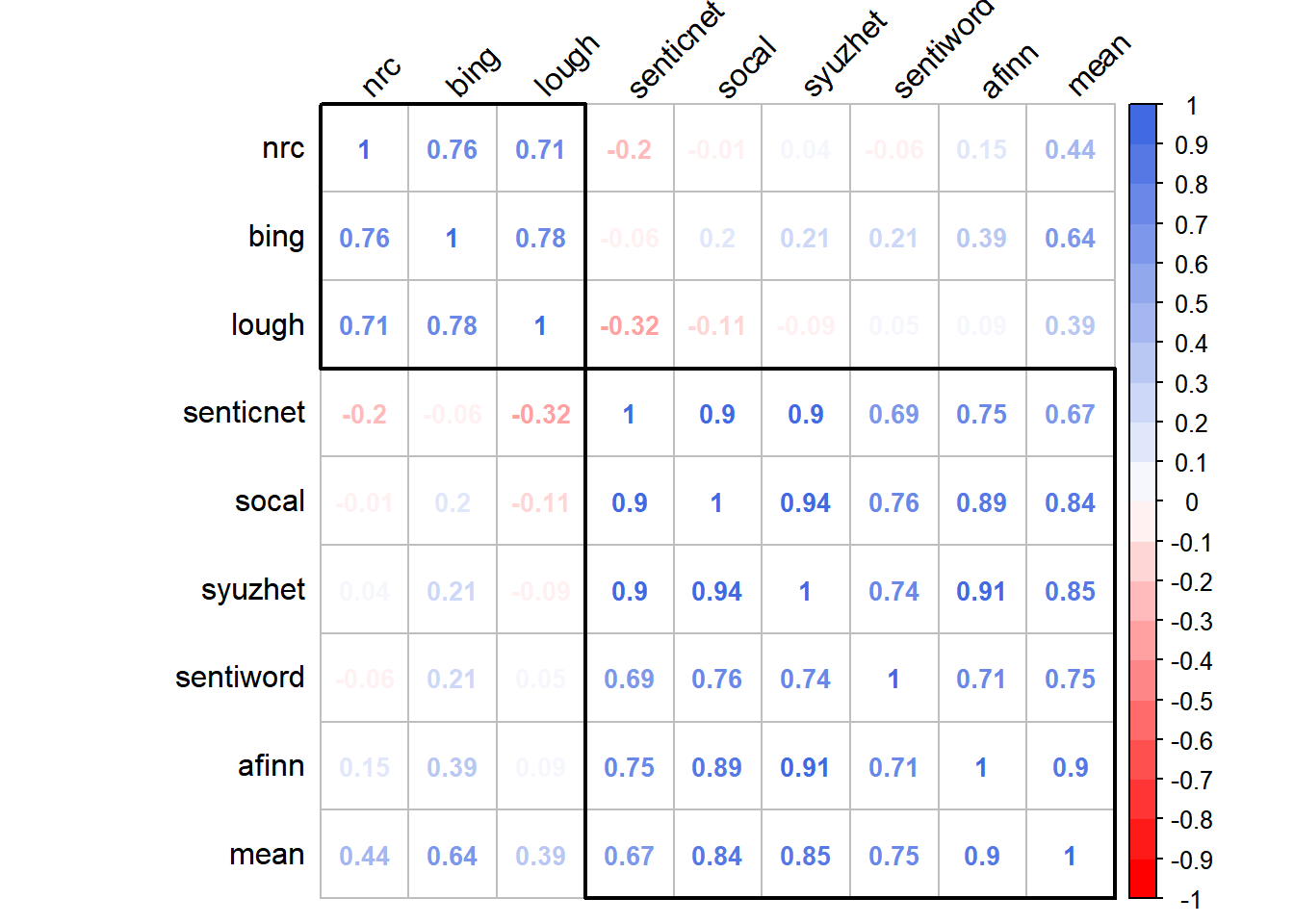 We see that the NRC, Bing and Loughran lexica are highly correlated with each other and less correlated with the other lexicons. Since these three lexica are all binary and the others are more finely graduated, this would probably explain this relationship.
4.8.1.2 Network Plots
These network plots were adapted from an excellent tutorial by Matt Dancho. Using thecorrr package shows the hidden structure and patterns in a more visual manner.
g_network_plot <- corr_matrix %>%
  corrr::network_plot(colours = c(palette_light()[[2]], "white", palette_light()[[4]]), legend = TRUE) +
  labs(title = "Correlations of Sentiment Lexica") +
  expand_limits(x = c(-0.5, 0.5), y = c(-0.5, 0.5)) +
  theme_tq() +
  theme(legend.position = "bottom")
g_network_plot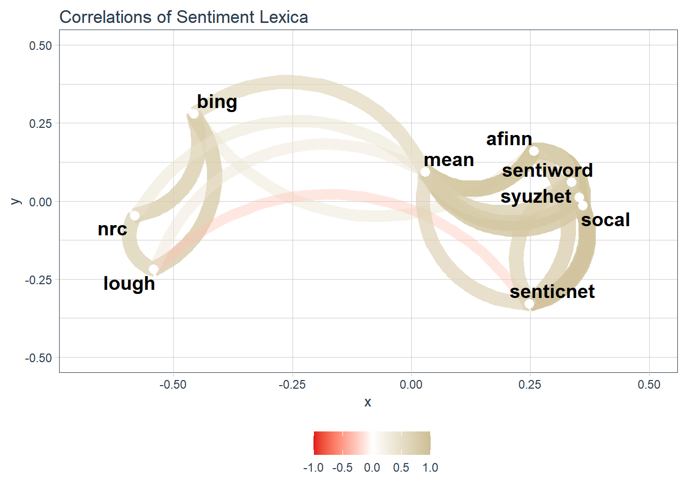
Since there are two distinctive groups of lexica, I’m going to redo the network graph without the mean variable included. It’s a slightly cleaner graph than the previous one.
# dataframe for correlation matrix
m2 <- brk_all_sentiment %>%
  select(-c(year, mean))

#correlation matrix
corr_matrix_m2 <- cor(m2)

g_network_plot_m2 <- corr_matrix_m2 %>%
  corrr::network_plot(colours = c(palette_light()[[2]], "white", palette_light()[[4]]), legend = TRUE) +
  labs(title = "Correlations of Sentiment Lexica Without Mean") +
  expand_limits(x = c(-0.5, 0.5), y = c(-0.5, 0.5)) +
  theme_tq() +
  theme(legend.position = "bottom")
g_network_plot_m2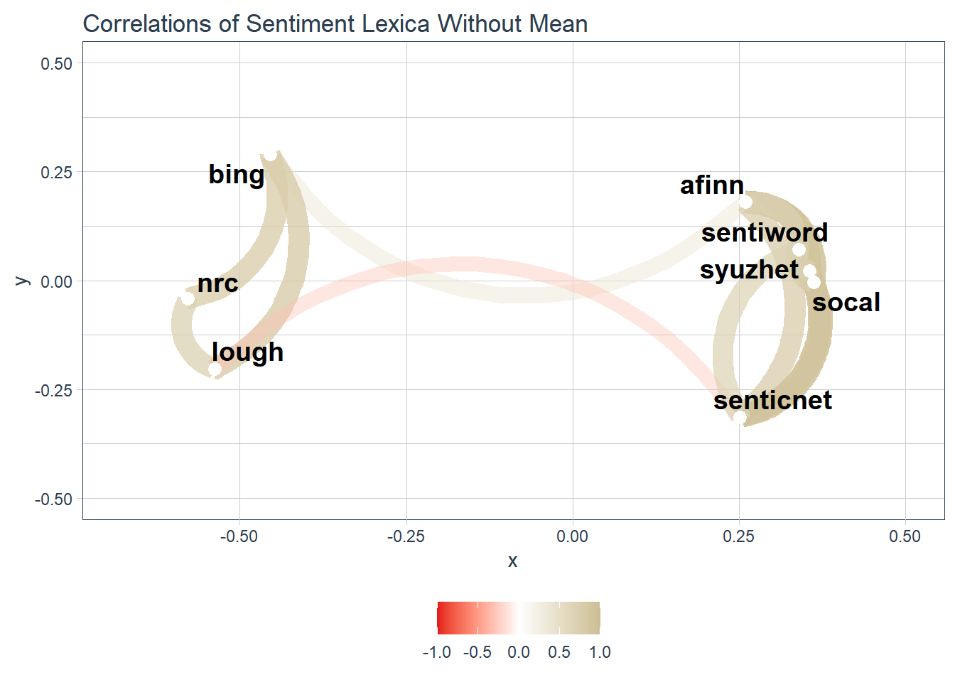
Since I’m exploring with different ways to visualize data, I’m going to chart all the different lexica over time. In the interests of time, I am going to do this in excel. First I will write the brk_all_sentiment dataframe to a csv file so I can read it into excel.
write.csv(brk_all_sentiment,"C:\\Users\\psonk\\Dropbox\\111 TC\\R stuff\\NLP\\berkshire\\brk_all_sentiment.csv", row.names = FALSE)Figure 4.8 shows a graph of all the lexica with the heavy red line being the average. This visualizes the correlation in a slightly different manner.
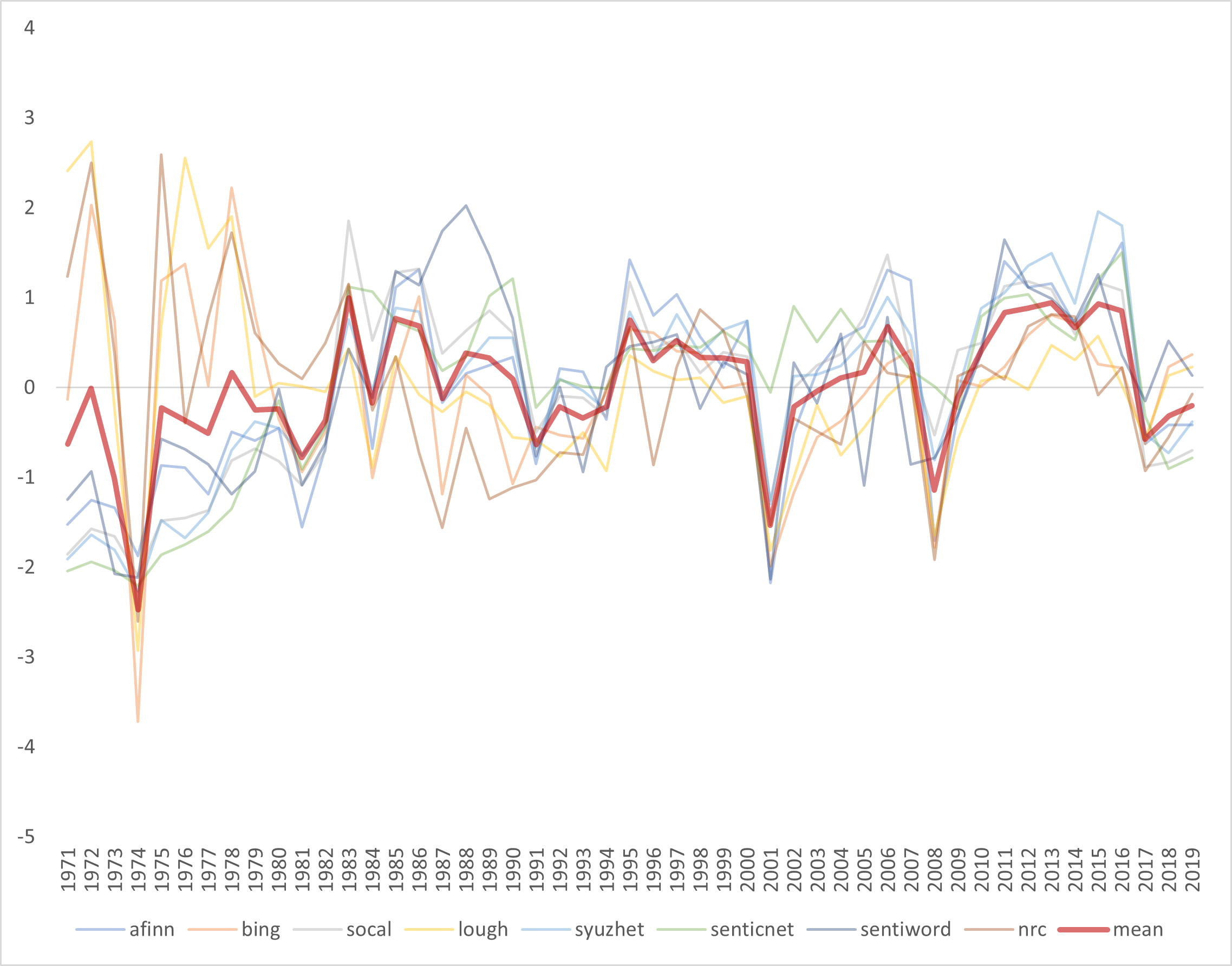
Figure 4.8: Graph of All Lexica
Figure 4.9 shows just the “binary” lexica (Bing, Loughran and NRC). We can see these are highly correlated.
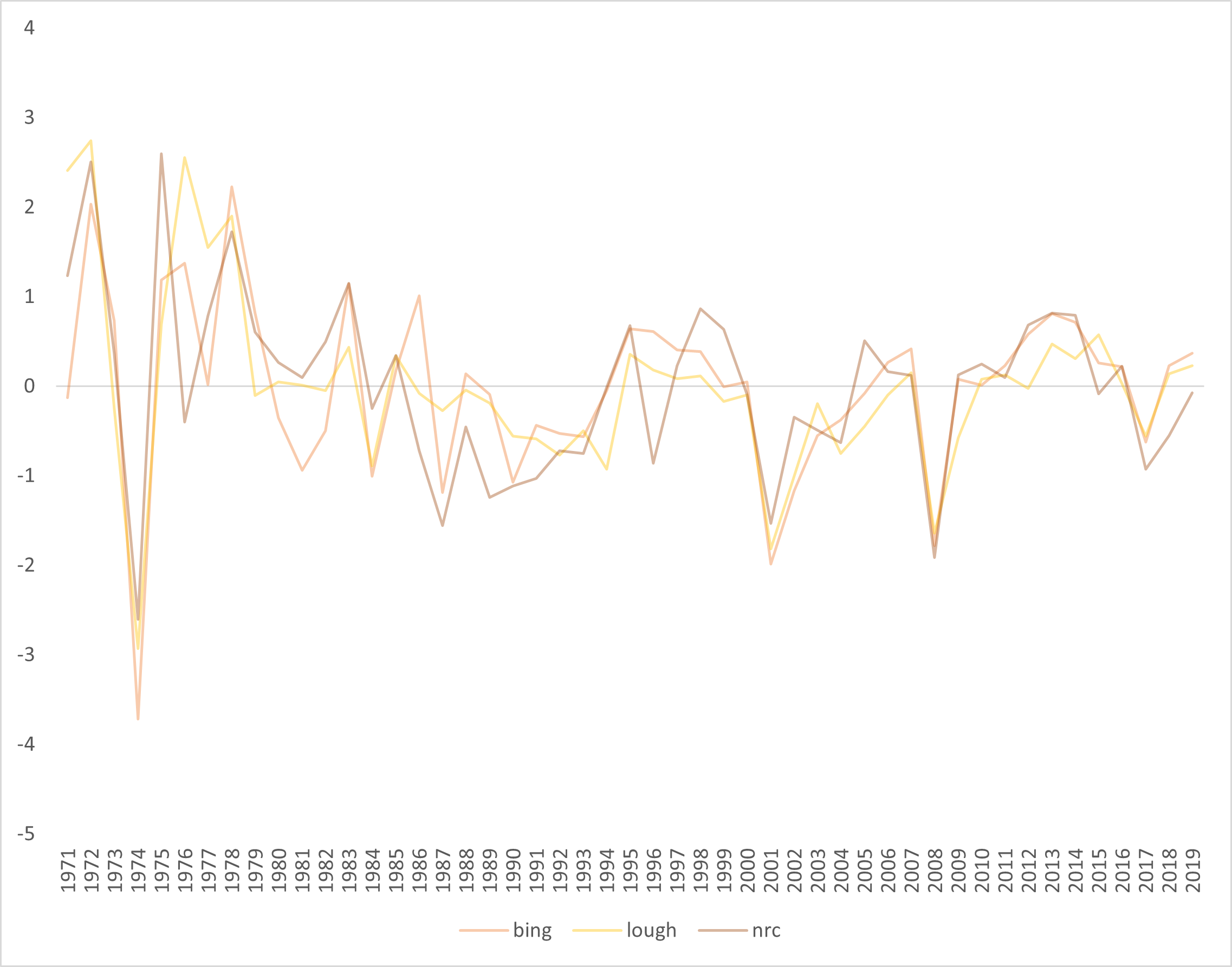
Figure 4.9: Graph of Binary Lexica
Figure 4.10 shows just the “continuous” lexica. We can see these are also highly correlated.
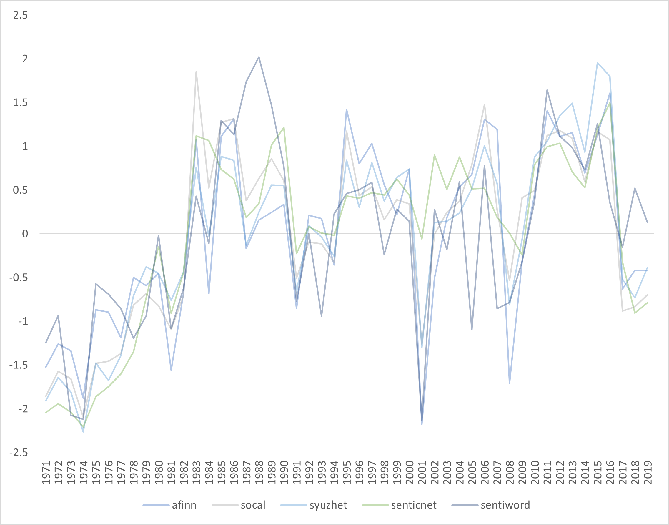
Figure 4.10: Graph of Binary Lexica
4.8.1.3 Nagging Worry
While the various lexica are pretty highly correlated, I have a nagging worry concerning the misclassification issues I discussed earlier. If they are all misclassifing in the same way, it might throw off my results when I perform regression analysis with Bershire’s returns.
| Try upset plots to show similarities between lexica UpSetR package |
| https://cran.r-project.org/web/packages/UpSetR/vignettes/queries.html |
No fancy code used, I just copied and pasted into a MS Word file↩︎
Update: I emailed Saif Mohammad and he agreed that it seemed strange that words would be classified as both. He gave me a thoughtful explanation as to how this can happen due to how the lexicon was compiled. He suggested I try another lexicon they created which includes intensity of emotions. I will add this to the list of things to follow up.↩︎