Chapter 6 Analysis of Sentiment vs. Peformance
6.1 Recap
To recap what we have done so far, in previous chapters we have:
- Chapter 2: Obtained and imported the letters into a dataframe.
- Chapter 3: Tokenized and cleaned the data.
- Chapter 4: Reviewed various sentiment lexica and merged with the letters.
- Chapter 5: Obtained, discussed and calculated various performance metrics.
Finally, after doing all that prep work we can compare sentiment to returns. To reiterate, it is unlikely that sentiment will be predictive of business or stock performance.
6.2 Creating Values for Average Sentiment of Binary and Continuous Lexica
Since some of the lexica are highly correlated and other are not, we will make averages of each group. avg_binary will be an average of the binary lexica (Bing, NRC and Loughran), while avg_continuous will be the average of the continuous lexica (AFINN, SO-CAL, Syuzhet, SenticNet and Sentiword).
#create average sentiment for binary and continuous lexica
brk_all_sentiment <- brk_all_sentiment %>%
  mutate(avg_binary = rowMeans(select(., bing, nrc, lough))) %>% #average of binary
  mutate(avg_continuous = rowMeans(select(.,-c(year, bing, nrc, lough)))) #average of continuous

brk_all_sentiment %>% print(n=5)
## # A tibble: 49 x 12
## year afinn bing socal lough syuzhet senticnet sentiword nrc mean avg_binary avg_continuous
## <dbl> <dbl> <dbl> <dbl> <dbl> <dbl> <dbl> <dbl> <dbl> <dbl> <dbl> <dbl>
## 1 1971 -1.52 -0.129 -1.86 2.41 -1.91 -2.04 -1.24 1.23 -0.631 1.17 -1.15
## 2 1972 -1.26 2.03 -1.57 2.74 -1.64 -1.94 -0.935 2.50 -0.00778 2.43 -0.703
## 3 1973 -1.34 0.733 -1.65 -0.245 -1.80 -2.04 -2.07 0.370 -1.01 0.286 -1.37
## 4 1974 -1.87 -3.72 -2.09 -2.93 -2.26 -2.21 -2.12 -2.60 -2.47 -3.08 -2.30
## 5 1975 -0.867 1.19 -1.48 0.691 -1.47 -1.86 -0.572 2.59 -0.222 1.49 -0.712
## # ... with 44 more rowsWe join these newley created data to the exisiting dataframe perf_and_sentiment.
perf_and_sentiment <- perf_data %>%
  left_join(brk_all_sentiment, by = "year")
6.3 Regressions
I’ll run ten pair-wise regressions. The two dependent variables will be the average sentiment measures: avg_binary and avg_continuous. The independent variables will be the five measures of performance (three absolute and two relative) discussed in the previous chapter:
Absolute measures of return: - sp500 is the annual return of the Standard & Poor’s 500 index. - book is the percentage change in Berkshire’s book value. - brk is the percentage change Berkshire’s stock price.
Relative measures of return: - alpha_book is book versus the sp500 which is the excess return of book value over the market - alpha_brk is brk versus the_sp500_ which is the excess return of stock price over the market
The next four sections will be:
- Binary sentiment lexica and absolute performance
- Continuous sentiment lexica and absolute performance
- Binary sentiment lexica and relative performance
- Continuous sentiment lexica and relative performance
6.3.1 Correlation of Binary Sentiment Lexica and Absolute Performance
I’m sure there is an easier way to do this but I’m just learning R. I’ll go through the first one step-by-step17 I first created a new dataframe scrap6 which contains just the the binary sentiment data and the absolute performance measures.
scrap6 <- perf_and_sentiment %>%
  select(year, brk, sp500, book, avg_binary, avg_continuous)

tibble(scrap6) %>% print(n=10)
## # A tibble: 49 x 6
## year brk sp500 book avg_binary avg_continuous
## <dbl> <dbl> <dbl> <dbl> <dbl> <dbl>
## 1 1971 0.805 0.146 0.164 1.17 -1.15
## 2 1972 0.081 0.189 0.217 2.43 -0.703
## 3 1973 -0.025 -0.148 0.047 0.286 -1.37
## 4 1974 -0.487 -0.264 0.055 -3.08 -2.30
## 5 1975 0.025 0.372 0.219 1.49 -0.712
## 6 1976 1.29 0.236 0.593 1.18 -0.806
## 7 1977 0.468 -0.074 0.319 0.784 -0.874
## 8 1978 0.145 0.064 0.24 1.95 -0.347
## 9 1979 1.02 0.182 0.357 0.439 -0.447
## 10 1980 0.328 0.323 0.193 -0.0111 -0.305
## # ... with 39 more rowsBut to plot these using facet_wrap I need to convert the dataframe to a “long form” using dplyr. This produces a dataframe with a separate row for each year by return type.
scrap6_long <- scrap6 %>%
  gather("brk", "sp500", "book", key = type, value = return) %>%
  relocate(type, .after = year) #move column
tibble(scrap6_long) %>% print(n=10)
## # A tibble: 147 x 5
## year type avg_binary avg_continuous return
## <dbl> <chr> <dbl> <dbl> <dbl>
## 1 1971 brk 1.17 -1.15 0.805
## 2 1972 brk 2.43 -0.703 0.081
## 3 1973 brk 0.286 -1.37 -0.025
## 4 1974 brk -3.08 -2.30 -0.487
## 5 1975 brk 1.49 -0.712 0.025
## 6 1976 brk 1.18 -0.806 1.29
## 7 1977 brk 0.784 -0.874 0.468
## 8 1978 brk 1.95 -0.347 0.145
## 9 1979 brk 0.439 -0.447 1.02
## 10 1980 brk -0.0111 -0.305 0.328
## # ... with 137 more rowsThen I feed these data into ggplot to produce the charts using various packages to format and make it look pretty. I was having trouble figuring out how to cross reference ggplot output in bookdown so I converted the plot to a png file using ggsave.
#create plot
g8 <- ggplot(scrap6_long, aes(x=avg_binary, y = return, color= type, label = year))+
  geom_text(check_overlap = T, size = 3) + #use year as datapoint instead of dot
  geom_smooth(method=lm, se = F) + #include regression line
  facet_wrap(~ type, nrow = 1, scales = "fixed",
             labeller = as_labeller(c(book = "Book Value", sp500 ="S&P 500 Index", brk = "Berkshire Stock" ))) +
  theme_bw() +
  theme(legend.position = "none") + #get rid of legend
  scale_y_continuous(labels = percent) +
  #ggpubr::stat_cor(label.y = -.7) + #use this code to include r and p-value in chart
  xlab("Binary Sentiment Score") +
  ylab("Return") +
    stat_cor(aes(label = paste(..rr.label.., ..p.label.., sep = "~`,`~")),
    label.y = -.7) #use this code to include r and p-value in chart

#ggplot in hi-res as png file
ggsave(g8, filename = "g8.png", dpi = 300, type = "cairo",
       width = 8, height = 6, units = "in")
lm1 <- lm(avg_binary ~ sp500, data= perf_and_sentiment)
summary(lm1)##
## Call:
## lm(formula = avg_binary ~ sp500, data = perf_and_sentiment)
##
## Residuals:
## Min 1Q Median 3Q Max
## -2.05711 -0.50945 -0.04085 0.40432 2.24596
##
## Coefficients:
## Estimate Std. Error t value Pr(>|t|)
## (Intercept) -0.3230 0.1402 -2.304 0.025684 *
## sp500 2.6604 0.6711 3.964 0.000249 ***
## ---
## Signif. codes: 0 '***' 0.001 '**' 0.01 '*' 0.05 '.' 0.1 ' ' 1
##
## Residual standard error: 0.7985 on 47 degrees of freedom
## Multiple R-squared: 0.2506, Adjusted R-squared: 0.2346
## F-statistic: 15.71 on 1 and 47 DF, p-value: 0.0002494I show the code I used to position the figure and cross reference below. Figure 6.1, shows correlation of
knitr::include_graphics("g8.png")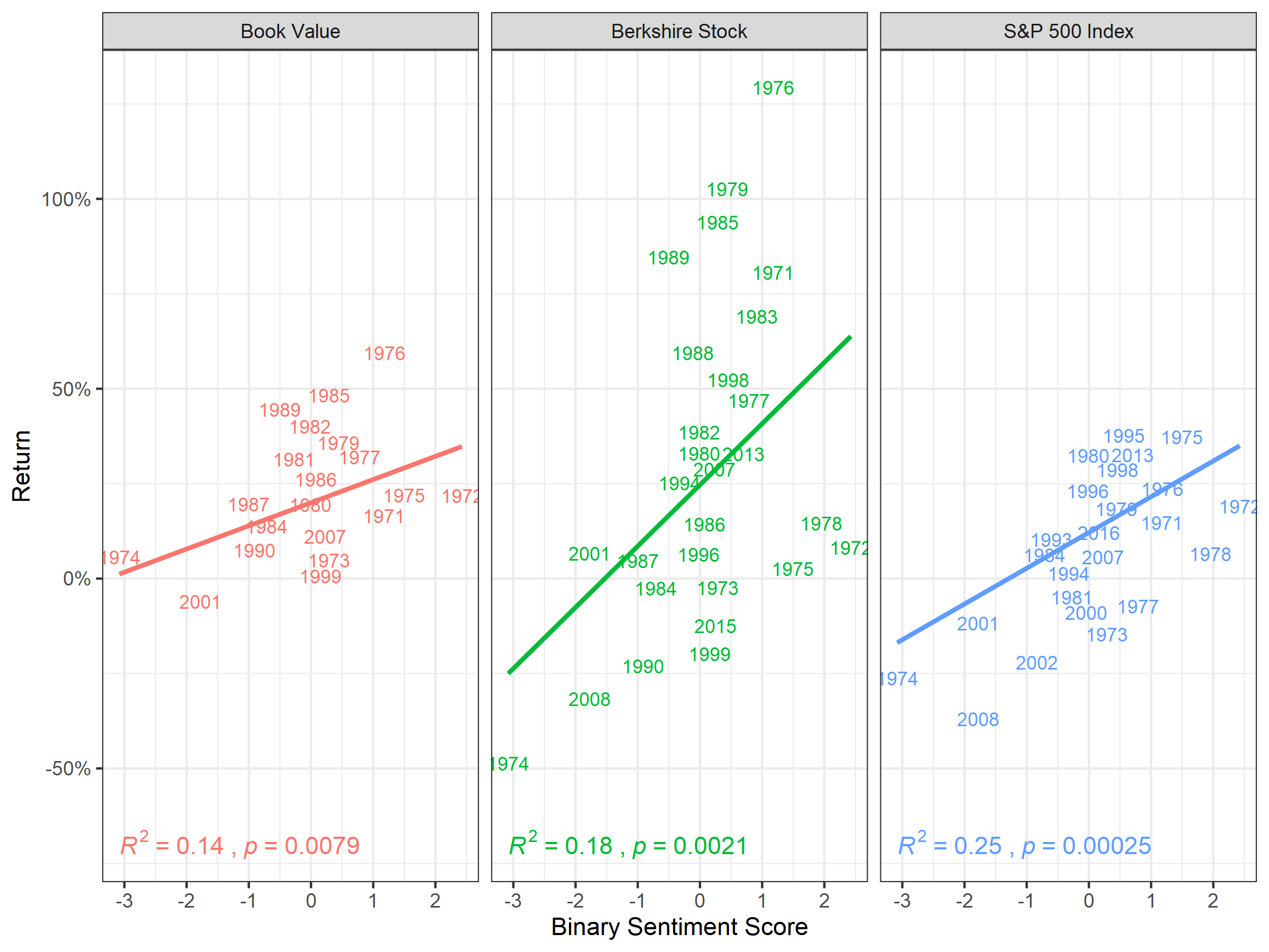
Figure 6.1: Correlation of Binary Sentiment Lexica and Absolute Performance
6.3.2 Correlation of Continuous Sentiment Lexica and Absolute Performance
In Figure 6.2, we see correlation of…
g9 <- ggplot(scrap6_long, aes(x=avg_continuous, y = return, color= type, label = year))+
  geom_text(check_overlap = T, size = 3) +
  geom_smooth(method=lm, se = F) + #include regression line
facet_wrap(~ type, nrow = 1, scales = "fixed",
             labeller = as_labeller(c(book = "Book Value", sp500 ="S&P 500 Index", brk = "Berkshire Stock" ))) +
  theme_bw() +
  theme(legend.position = "none") + #get rid of legend
  scale_y_continuous(labels = percent)  +
  stat_cor(aes(label = paste(..rr.label.., ..p.label.., sep = "~`,`~")),
    label.y = -.7) +
  xlab("Average Continuous Sentiment Score") +
  ylab("Return")

#ggplot in hi-res as png file
ggsave(g9, filename = "g9.png", dpi = 300, type = "cairo",
       width = 8, height = 6, units = "in")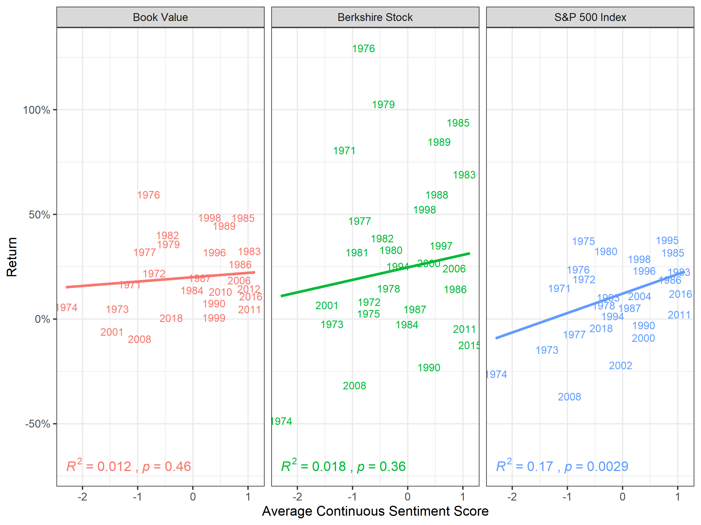
Figure 6.2: Correlation of Continuous Sentiment Lexica and Absolute Performance
6.3.3 Correlation of Binary Sentiment Lexica and Relative Performance
In Figure 6.3, we see correlation of…
#create new dataframe "scrap6"
scrap7 <- perf_and_sentiment %>%
  select(year, alpha_brk, alpha_book, avg_binary, avg_continuous)
# convert to long form using "gather" and create new dataframe "scrap6_long"
scrap7_long <- scrap7 %>%
  gather("alpha_brk", "alpha_book", key = type, value = return)

g10 <- ggplot(scrap7_long, aes(x=avg_binary, y = return, color= type, label = year))+
  geom_text(check_overlap = T, size = 3) +
  geom_smooth(method=lm, se = F) + #include regression line
  facet_wrap(~ type, nrow = 1, scales = "fixed",
             labeller = as_labeller(c(alpha_book = "Berkshire Book Value Excess Return over S&P 500", alpha_brk ="Berkshire Stock Excess Return over S&P 500")))+
  theme_bw() +
  theme(legend.position = "none") + #get rid of legend
  scale_y_continuous(labels = percent) +
  ggpubr::stat_cor(aes(label = paste(..rr.label.., ..p.label.., sep = "~`,`~")),
    label.y = -.5)+
  xlab(" Binary Sentiment Score") +
  ylab("Return")

#ggplot in hi-res as png file
ggsave(g10, filename = "g10.png", dpi = 300, type = "cairo",
       width = 8, height = 6, units = "in")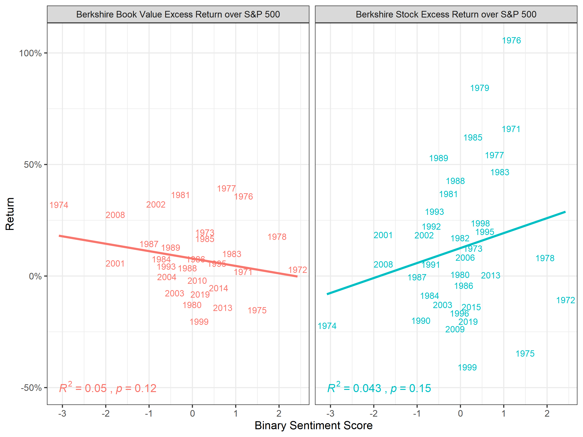
Figure 6.3: Correlation of Binary Sentiment Lexica and Relative Performance
6.3.4 Correlation of Continuous Sentiment Lexica and Relative Performance
In Figure 6.4, we see correlation of…
g11 <- ggplot(scrap7_long, aes(x=avg_continuous, y = return, color= type, label = year))+
  geom_text(check_overlap = T, size = 3) +
  geom_smooth(method=lm, se = F) + #include regression line
  facet_wrap(~ type, nrow = 1, scales = "fixed",
             labeller = as_labeller(c(alpha_book = "Berkshire Book Value Excess Return over S&P 500", alpha_brk ="Berkshire Stock Excess Return over S&P 500")))+
  theme_bw() +
  theme(legend.position = "none") + #get rid of legend
  scale_y_continuous(labels = percent) +
  ggpubr::stat_cor(aes(label = paste(..rr.label.., ..p.label.., sep = "~`,`~")),
    label.y = -.5)+
  xlab("Continuous Sentiment Score") +
  ylab("Return")

#ggplot in hi-res as png file
ggsave(g11, filename = "g11.png", dpi = 300, type = "cairo",
       width = 8, height = 6, units = "in")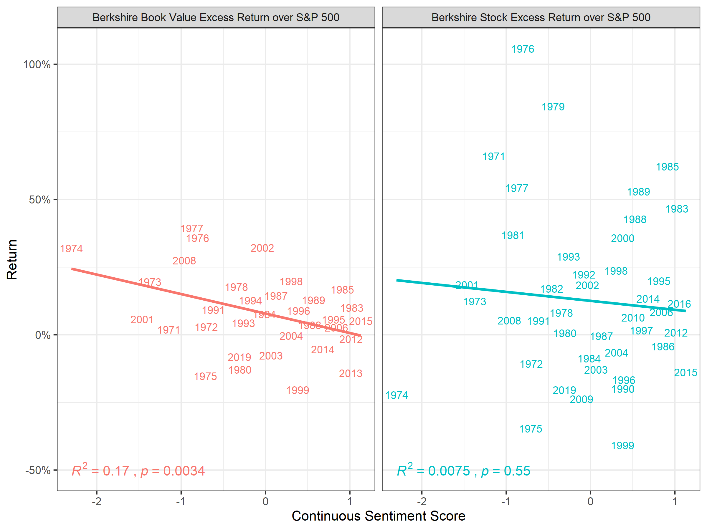
Figure 6.4: Correlation of Continuous Sentiment Lexica and Relative Performance
Alternative format for charts from the ggpubr package
#cool charts from ggpubr package
g12 <- ggscatter(
  scrap6_long, x = "avg_binary", y = "return",
  color = "type",
  add = "reg.line") +
  scale_y_continuous(labels = percent) +
  facet_wrap(~ type, nrow = 1, scales = "fixed",
             labeller = as_labeller(c(book = "Book Value", sp500 ="S&P 500 Index", brk = "Berkshire Stock" ))) +
  ggpubr::stat_cor(aes(label = paste(..rr.label.., ..p.label.., sep = "~`,`~")),
    label.y = -.6)+
  theme(legend.position = "none") +
  xlab("Average Binary Sentiment Score") +
  ylab("Return")

#ggplot in hi-res as png file
ggsave(g12, filename = "g12.png", dpi = 300, type = "cairo",
       width = 8, height = 6, units = "in")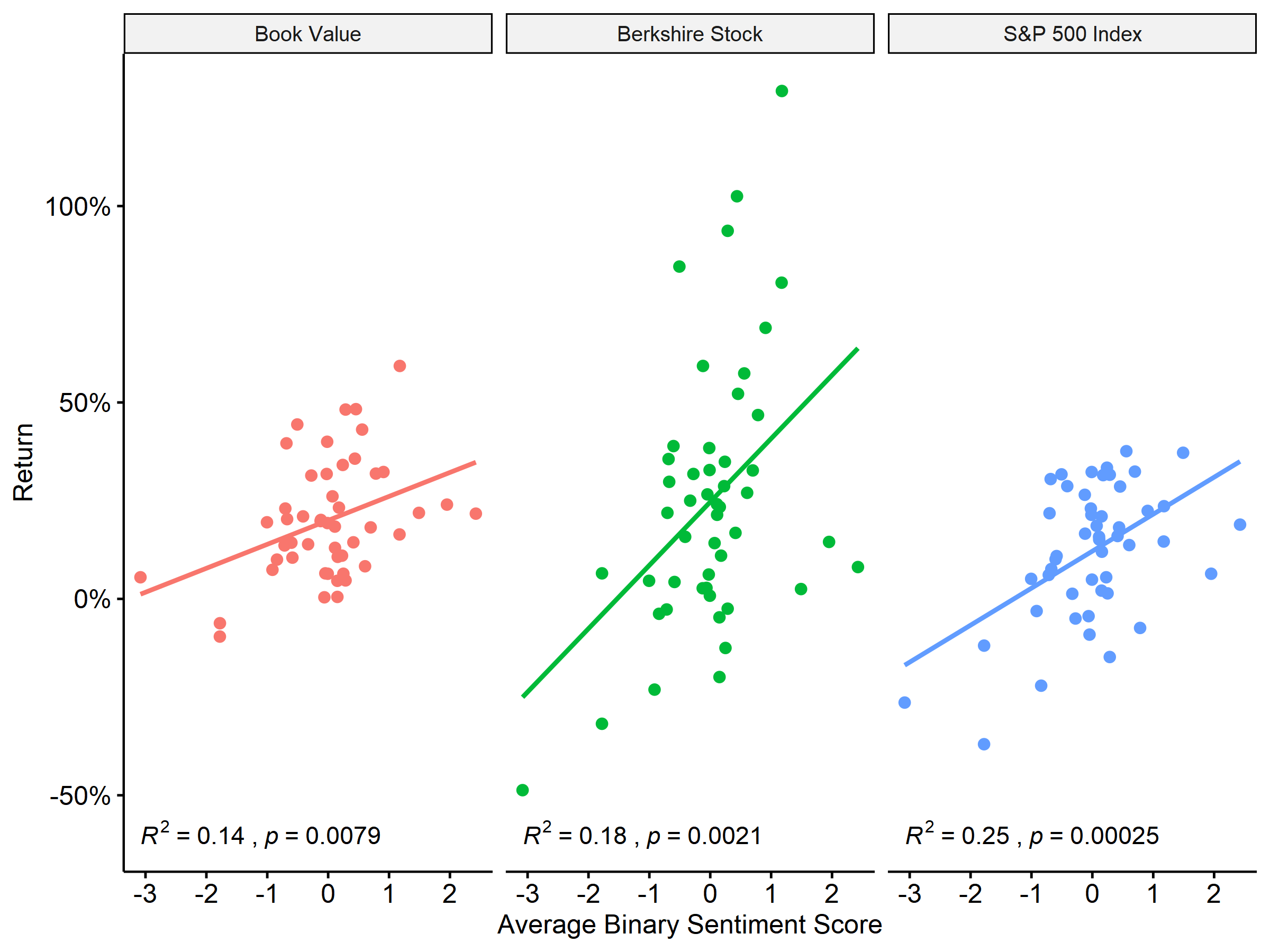
Figure 6.5: Correlation of Binary Sentiment Lexica and Relative Performance Measures
6.4 Discussion of Results
scrap8 <-  perf_data %>%
  arrange(desc(alpha_book))

#gt(scrap8[1:10,])%>%
#  fmt_percent(
#    columns = 2:6,
#    decimals = 1) %>%
#    tab_header(title = "Berkshire Performance and Sentiment")

scrap9 <- perf_and_sentiment %>%
  select(year, brk, sp500, book, alpha_brk, alpha_book, avg_binary, avg_continuous)

DT::datatable(scrap9) %>%
  formatPercentage(columns = 2:6, digits = 1) %>%
  formatRound(columns = 7:8, digits = 1)
#DT::datatable(perf_data) %>%
# formatPercentage(columns = 2:6, digits = 1)6.5 Examination of Residuals and Assumptions for Linear Regression
Basically so I can remember what I did when I refer back to this months from now.↩︎