Chapter 5 Importing and Processing of Performance Data
5.1 Measures of Berkshire’s Performance
Now that we have sentiment data for Berkshire’s letters, it would be interesting to combine it with Berkshire’s performance data to see if there are any correlations. As I mentioned previously, it is unlikely that sentiment will be predictive of business or stock performance. At best, it is likely a coincident indicator. But that being said, what metric should we use to measure Berkshire’s performance? What performance measures might influence Buffett’s sentiment when he is writing the letters? The answer isn’t straightforward and we actually have a few different measures to look at.
5.2 A Little Background on Buffett’s Choice of Perfomance Metrics
You might think the obvious choice is the annual return of Berkshire stock. But this actually wasn’t what I thought of first. You see, Buffett historically didn’t really measure himself by the moves in Berkshire’s stock price. He feels that the stock market is “…there to serve you” and that “…you can ignore it…” Someone who thinks like this wouldn’t judge themselves by stock performance. Buffett views on the irrationality of the stock market can be traced to the end of Chapter 8 of The Intelligent Investor (first published in 1949) where Ben Graham14 talks about “Mr. Market,” his personification of the stock market:
Let us close this section with something in the nature of a parable. Imagine that in some private business you own a small share that cost you $1,000. One of your partners, named Mr. Market, is very obliging indeed. Every day he tells you what he thinks your interest is worth and furthermore offers either to buy you out or to sell you an additional interest on that basis. Sometimes his idea of value appears plausible and justified by business developments and prospects as you know them. Often, on the other hand, Mr. Market lets his enthusiasm or his fears run away with him, and the value he proposes seems to you a little short of silly.
If you are a prudent investor or a sensible businessman, will you let Mr. Market’s daily communication determine your view of the value of a $1,000 interest in the enterprise? Only in case you agree with him, or in case you want to trade with him. You may be happy to sell out to him when he quotes you a ridiculously high price, and equally happy to buy from him when his price is low. But the rest of the time you will be wiser to form your own ideas of the value of your holdings, based on full reports from the company about its operations and financial position (Graham 1973).
Buffett often tells the story of “Mr. Market” with a little more color than the original. Here is what Buffett said in a 2015 interview.
“The nice thing about it [the market] is this imaginary person out there – Mr. Market – is kind of a drunken psycho. Some days he gets very enthused and some days he gets very depressed. And when he get really enthused, if you happen to be trading stocks you sell to him and if he gets depressed you buy from him” (Gilbert and Farner 2015).
We also have to factor in some context into how Buffett developed these views. When he worked for Graham-Newman from 1951 to 1956, Ben Graham often trafficked in “secondary issues” or stocks and bonds that traded in the “over-the-counter” market, not on organized exchanges like the New York Stock Exchange. These securities in many cases were extremely illiquid and the quoted price was often not an indication of the security’s true “intrinsic value.” In the Buffett Partnership, which Buffett ran from 1956 to 1969, much of the portfolio was in these types of illiquid securities. Buffett started buying Berkshire in 1964 and until the mid-1970 it traded in the “Pink Sheets.” In 1994 while I was in business school, I did a project for my security analysis class and analyzed Berkshire. When I went back to find historic prices, I notice that in the late 1960s and early 1970s, the stock didn’t trade for weeks at a time - it was extremely illiquid.
The bottom line is that given his education and experience, we actually wouldn’t expect Buffett to use Berkshire’s stock price as a measure of performance.
5.3 How Buffett Measured His Own Perfomance Over Time
So if Buffett didn’t gauge his performance with Berkshire’s stock return, what metric did he use? This isn’t a simple answer as it has changed a few times over the past 50 years. In the 1971 letter (the first one penned by him), Buffett uses operating earnings and return on equity to judge Berkshire’s performance. This was the metric he used until 1983 when he switched to measuring performance by changes in book value. In the 1983 letter he states the reason why. While he provides a longer explanation in the letter, here is a brief excerpt:
We report our progress in terms of book value because in our case (though not, by any means, in all cases) it is a conservative but reasonably adequate proxy for growth in intrinsic business value - the measurement that really counts. (Buffett 1983).
Buffett started including a table of Berkshire’s performance (as measured by changes in book value) versus the S&P 500 at some point before 199615. Figure 5.1 shows the table which included percent change in per share book value, percent change in the S&P 500 and the difference.
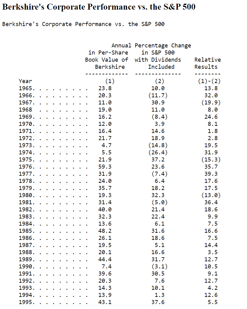
Figure 5.1: Performance Table from 1995 Annual Report
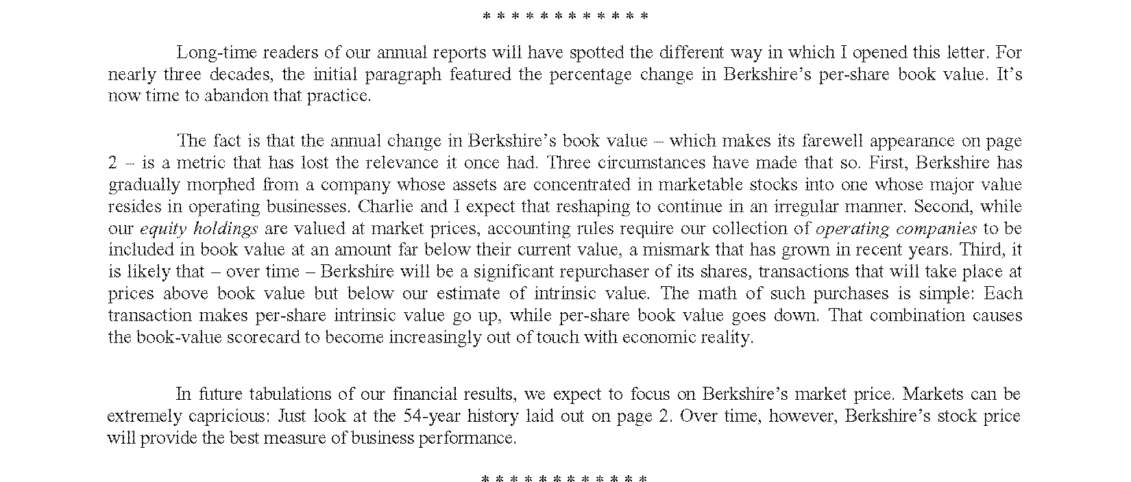
Figure 5.2: Performance Table from 1995 Annual Report
It is clear that for over 50 years, Buffett did not use Berkshire’s stock price to measure his performance. Rather, he used book value per share with the S&P 500 as a benchmark. We will use all of these metrics and see which ones, if any, correlate with sentiment.
5.4 Distinction Between Absolute and Relative Performance
There is an important distinction to be made between measures of absolute and relative performance because the effect on sentiment can be significant. Absolute return is simply the return generated over a given period. Relative return is the difference between absolute return and a benchmark such as the S&P 500. In finance, relative return is also called alpha. If a portfolio manager is “beating the market” or “producing alpha” that means his absolute return is more than the market. It should be noted that one can have negative absolute return but still generate alpha. For example, if the S&P 500 is down 20% but your portfolio is down 10% you have generated 1000 basis points of alpha. Yet another expression for alpha is “excess return.” I will use these interchangeably.
Buffett in his letters used book value as an absolute return measure, the S&P 500 as his benchmark and reported relative return of book versus the S&P. Alpha is a simple formula:
alpha = absolute return - benchmark
for Berkshire, as shown in Figure 5.1, this was…
relative results = annual percent change in per-share book value - annual percent change in S&P 500 with dividends included
We will have three variables which measure absolute return:
- sp500 is the annual return of the Standard & Poor’s 500 index.
- book is the percentage change in Berkshire’s book value
- brk is the percentage change Berkshire’s stock price
And two variables which capture relative return:
- alpha_book is book versus the sp500 which is the excess return of book value over the market
- alpha_brk is brk versus the_sp500_ which is the excess return of stock price over the market
5.5 Obtain and Import Perfomance Data
Data were taken from the 2018 (just book value) and 2019 annual report (stock and market return). These were copied to an excel spreadsheet and imported into a dataframe perf_data using this code. I used the package kable and kabelExtra to make the html tables as shown in Table 5.1.
#read in performance data
perf_data = read.csv("C:\\Users\\psonk\\Dropbox\\111 TC\\R stuff\\NLP\\berkshire\\performance since 1971.csv")
#change name of column
names(perf_data)[1] <- "year"
#change "year" column from character to numeric
perf_data$year <- as.numeric(perf_data$year)
#cool html table
kable(perf_data[1:5,], caption = "Berkshire Performance Metrics") %>%
kable_styling(bootstrap_options = c("striped", "hover", "condensed"))| year | brk | sp500 | alpha_brk | book | alpha_book |
|---|---|---|---|---|---|
| 1971 | 0.805 | 0.146 | 0.659 | 0.164 | 0.018 |
| 1972 | 0.081 | 0.189 | -0.108 | 0.217 | 0.028 |
| 1973 | -0.025 | -0.148 | 0.123 | 0.047 | 0.195 |
| 1974 | -0.487 | -0.264 | -0.223 | 0.055 | 0.319 |
| 1975 | 0.025 | 0.372 | -0.347 | 0.219 | -0.153 |
5.6 Correlation of Performance Measures
5.6.1 Overall Correlation
Figure 5.3 shows the correlation matrix for performance measures. The correlation of between Berkshire’s stock and the S&P 500 (both absolute return measures) at 0.51 is no surprise. Also, since a large portion of Berkshire’s book value historically has been in US equities, we would also expect book value to be correlated to the S&P 500 (also absolute return measures) which it is at 0.65.
# ggpairs correlation matrix
corr_for_perf <- ggpairs(perf_data, columns = c("brk", "sp500", "alpha_brk", "book", "alpha_book"))

# ggpairs correlation matrix in hi-res
ggsave(corr_for_perf, filename = "corrforperf.png", dpi = 300, type = "cairo",
       width = 8, height = 6, units = "in")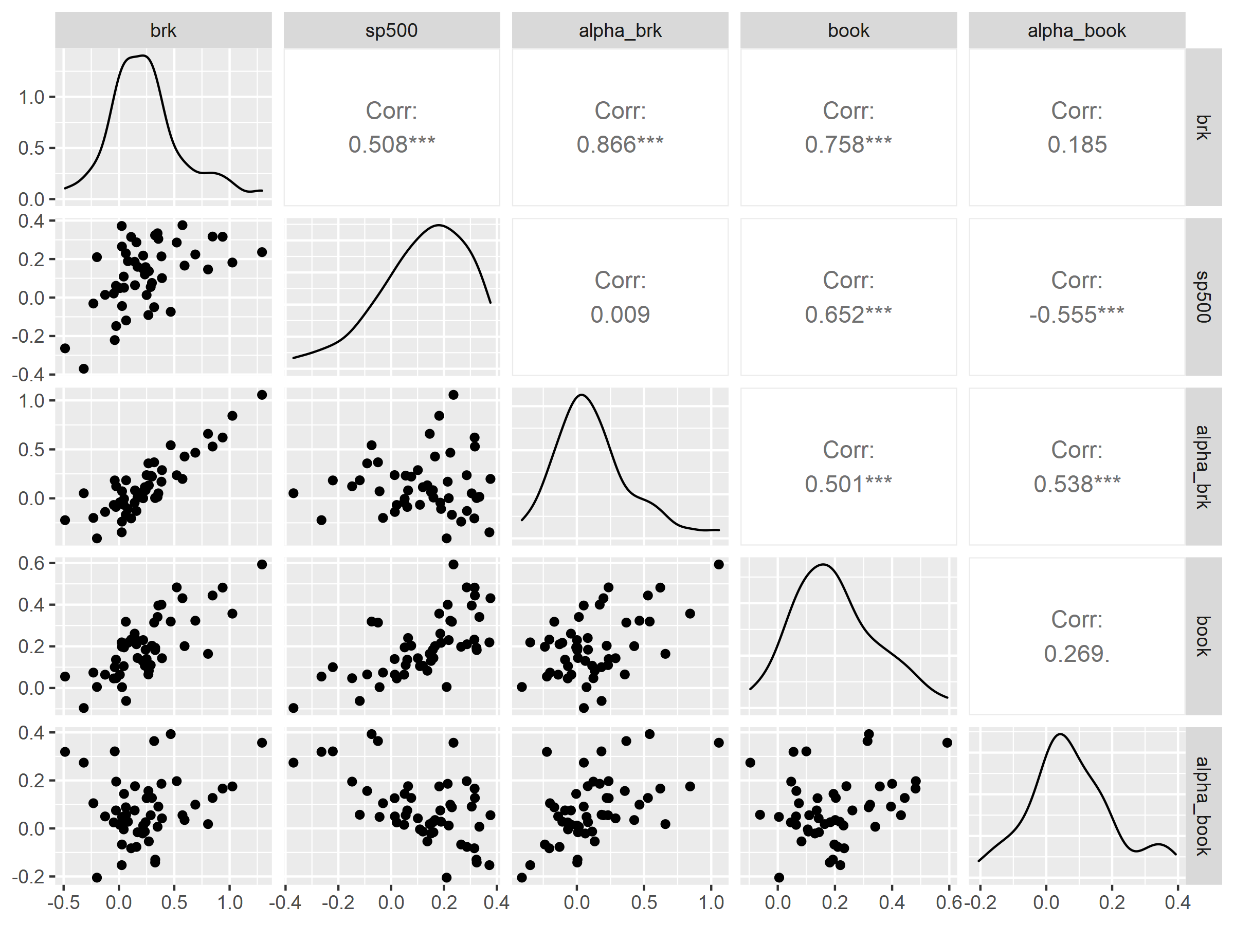
Figure 5.3: Correlation of Measures of Berkshire’s Performance
Again, while one could eyeball the matrix and see correlations, using hierarchical clustering order in the corrplot package really makes this relationship jump out. We see the correlation between the S&P 500 and book value (absolute) in one cluster in Figure 5.4. In the other cluster, we see correlations of Berkshire stock price (absolute) and alpha of book as well as alpha of stock over S&P 500 (both relative). What is interesting is the negative correlation of alpha of book versus the S&P 500 (relative).
# dataframe for correlation matrix
m_perf <- perf_data %>%
  select(-c(year))

#correlation matrix
corr_matrix_perf <- cor(m_perf)
#as_tibble(corr_matrix)

#nicer colors
col<- colorRampPalette(c("red", "white", "royalblue"))(20)

#correlation matrix with h clustering
corrplot::corrplot(corr_matrix_perf, method = "number", order = "hclust", addrect = 2, tl.col = "black", tl.srt = 45, col = col, number.cex=.85 )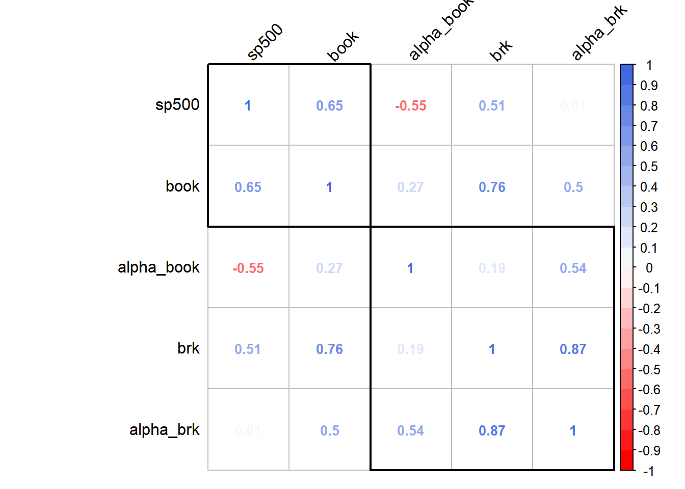
Figure 5.4: Hierarchical Clustering of Correlation of Berkshire’s Performance
The network plot in Figure 5.5 shows these correlations in an even more visual way.
g_network_plot_perf <- corr_matrix_perf %>%
  corrr::network_plot(colours = c(palette_light()[[2]], "white", palette_light()[[4]]), legend = TRUE) +
  labs(title = NULL, x = NULL, y = NULL) +
  expand_limits(x = c(-0.5, 0.5), y = c(-0.5, 0.5)) +
  theme_tq() +
  theme(legend.position = "bottom")
g_network_plot_perf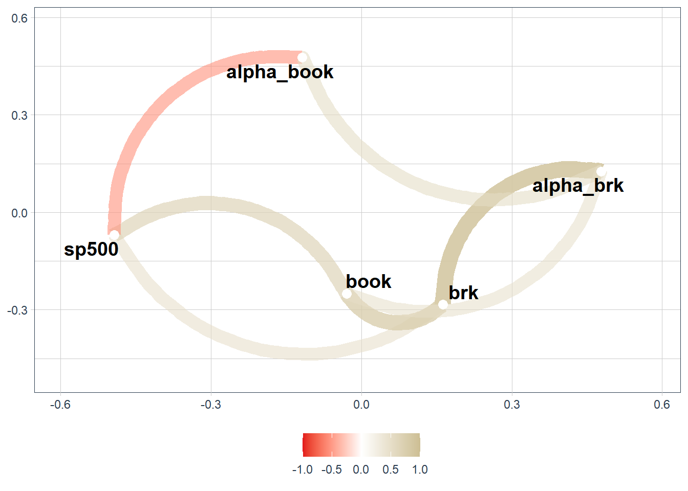
Figure 5.5: Network Plot of Correlation of Berkshire’s Performance
5.6.2 Negative Correlation Between alpha_book and sp500
I wanted to explore the negative correlation of -0.55 between alpha_book and the S&P 500. As a reminder, book value is the primary measure Buffett uses to gauge his performance and he uses the S&P 500 as a benchmark so his performance would be:
alpha_book = change in book value - change in S&P 500 = excess return over S&P 500
The chart in Figure 5.6 shows the regression of sp500 on alpha_book. What this shows is that Buffett tended to generate huge alpha in years when the S&P was negative and less alpha when the S&P was positive.
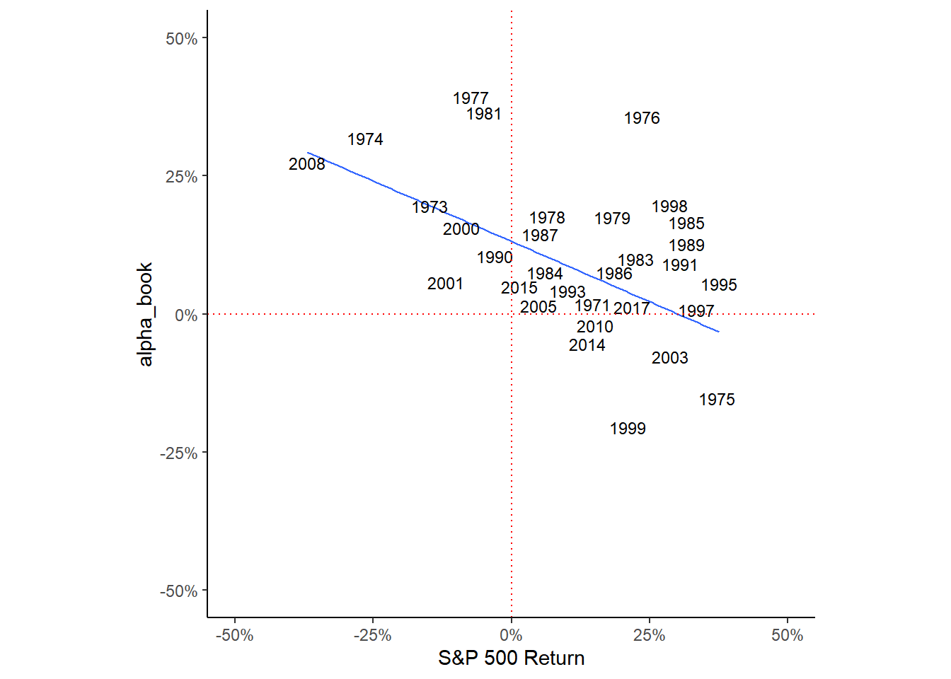
Figure 5.6: Network Plot of Correlation of Berkshire’s Performance
As a value investor, this kind of makes sense, you outperform over time by not loosing money. As shown in Table 5.2, Berkshire only had a decrease in book value twice - in 2001 and 2008 - and in both years did better than the S&P 500.
| year | book | sp500 | alpha_book |
|---|---|---|---|
| 2001 | -0.062 | -0.119 | 0.057 |
| 2008 | -0.096 | -0.370 | 0.274 |
Not losing money is the guiding principle of all value investors. Buffett is often quoted as saying:
The first rule in investment is don’t lose. And the second rule in investment is don’t forget the first rule, and that’s all the rules there are. If you buy things for far below what they’re worth, and you buy a group of them, you basically don’t lose money (Buffett 1985).
5.7 Brief Discussion of Performance and Possible Relationship with Sentiment
An analysis of Berkshire’s performance is beyond the scope of this project. The only reason for discussing it is the effect it might have on sentiment. The purpose of these letters is to communicate to shareholders the results of the previous year and the outlook going forward16. Berkshire usually releases its year end letter in the last week of February. The sentiment valence in the letter is obviously influence heavily by the performance in the previous year and the outlook going forward. But outlook could also be influenced by developments between the year end and the date the letter is released. It would be interesting to see if the performance of the S&P 500 between January 1 and February 28 is correlated. This might influence outlook at this is what the market is doing while Buffett is writing the letter. We could also look at changes in book value in the first quarter which ends March 31st which would give us a window into how the businesses are performing while he is writing the letter.
5.8 Combining Performance and Sentiment Data
Finally, we combine the performance data with sentiment data to produce a dataframe perf_and_sentiment as shown in Table ??
#change to numeric to join
brk_all_sentiment$year <- as.numeric(brk_all_sentiment$year)
#colnames(brk_all_sentiment)

#left join and create new dataframe "perf_and_sentiment"
perf_and_sentiment <- perf_data %>%
  left_join(brk_all_sentiment, by = "year")

gt(perf_and_sentiment[1:5,])%>%
  fmt_percent(
    columns = 2:6,
    decimals = 1) %>%
  fmt_number(
    columns = 7:15,
    decimals = 1,
    suffixing = TRUE) %>%
tab_header(title = "Berkshire Performance and Sentiment")| Berkshire Performance and Sentiment | ||||||||||||||
|---|---|---|---|---|---|---|---|---|---|---|---|---|---|---|
| year | brk | sp500 | alpha_brk | book | alpha_book | afinn | bing | socal | lough | syuzhet | senticnet | sentiword | nrc | mean |
| 1971 | 80.5% | 14.6% | 65.9% | 16.4% | 1.8% | −1.5 | −0.1 | −1.9 | 2.4 | −1.9 | −2.0 | −1.2 | 1.2 | −0.6 |
| 1972 | 8.1% | 18.9% | −10.8% | 21.7% | 2.8% | −1.3 | 2.0 | −1.6 | 2.7 | −1.6 | −1.9 | −0.9 | 2.5 | −0.0 |
| 1973 | −2.5% | −14.8% | 12.3% | 4.7% | 19.5% | −1.3 | 0.7 | −1.7 | −0.2 | −1.8 | −2.0 | −2.1 | 0.4 | −1.0 |
| 1974 | −48.7% | −26.4% | −22.3% | 5.5% | 31.9% | −1.9 | −3.7 | −2.1 | −2.9 | −2.3 | −2.2 | −2.1 | −2.6 | −2.5 |
| 1975 | 2.5% | 37.2% | −34.7% | 21.9% | −15.3% | −0.9 | 1.2 | −1.5 | 0.7 | −1.5 | −1.9 | −0.6 | 2.6 | −0.2 |
Now we can finally examine the relationship between sentiment and performance.
Benjamin Graham is considered “The Dean of Value Investing” and was Buffett’s professor at Columbia Business School. Upon graduation in 1951, Buffett worked for Graham until Graham’s retirement in 1956.↩︎
I can’t seem to find annual reports before 1995 online and the letters to shareholders do not include the table↩︎
In terms of areas for further research, I can use the LIWC lexicon to examine forward versus backward looking language↩︎