#> [1] 0.00 0.15 0.40 0.45 0.002 Small and Large Worlds
ORIGINAL
Learning Objectives
“This chapter focuses on the small world. It explains probability theory in its essential form: counting the ways things can happen. Bayesian inference arises automatically from this perspective. Then the chapter presents the stylized components of a Bayesian statistical model, a model for learning from data. Then it shows you how to animate the model, to produce estimates.
All this work provides a foundation for the next chapter, in which you’ll learn to summarize Bayesian estimates, as well as begin to consider large world obligations.” (McElreath, 2020, p. 20) (pdf)
The text references many times to the notions of small and large worlds:
- The small world is the self-contained logical world of the model.
- The large world is the broader context in which one deploys a model.
TIDYVERSE
The work by Solomon Kurz has many references to R specifics, so that people new to R can follow the course. Most of these references are not new to me, so I will not include them in my personal notes. There are also very important references to other relevant articles I do not know. But I will put these kind of references for now aside and will me mostly concentrate on the replication and understanding of the code examples.
One challenge for Kurz was to replicate all the graphics of the original version, even if they were produced just for understanding of procedures and argumentation without underlying R code. By contrast I will use only those code lines that are essential to display Bayesian results. Therefore I will not replicate for example the very extensive explication how to produce with tidyverse means the graphics of the garden of forking data.
2.1 The Garden of Forking Data
2.1.1 ORIGINAL
Bayesian inference is counting of possibilities
“Bayesian inference is really just counting and comparing of possibilities.” (McElreath, 2020, p. 20) (pdf)
“In order to make good inference about what actually happened, it helps to consider everything that could have happened. A Bayesian analysis is a garden of forking data, in which alternative sequences of events are cultivated. As we learn about what did happen, some of these alternative sequences are pruned. In the end, what remains is only what is logically consistent with our knowledge.” (McElreath, 2020, p. 21) (pdf)
2.1.1.1 Counting possibilities
“Suppose there’s a bag, and it contains four marbles. These marbles come in two colors: blue and white. We know there are four marbles in the bag, but we don’t know how many are of each color. We do know that there are five possibilities: (1) [⚪⚪⚪⚪], (2) [⚫⚪⚪⚪], (3)[⚫⚫⚪⚪], (4) [⚫⚫⚫⚪], (5) [⚫⚫⚫⚫]. These are t These These are the only possibilities consistent with what we know about the contents of the bag. Call these five possibilities the conjectures.
Our goal is to figure out which of these conjectures is most plausible, given some evidence about the contents of the bag. We do have some evidence: A sequence of three marbles is pulled from the bag, one at a time, replacing the marble each time and shaking the bag before drawing another marble. The sequence that emerges is: ⚫⚪⚫, in that order. These are the data.
So now let’s plant the garden and see how to use the data to infer what’s in the bag. Let’s begin by considering just the single conjecture, [ ], that the bag contains one blue and three white marbles.” (McElreath, 2020, p. 21) (pdf)
| Conjecture | Ways to produce ⚫⚪⚫ |
| [⚪⚪⚪⚪] | 0 × 4 × 0 = 0 |
| [⚫⚪⚪⚪] | 1 × 3 × 1 = 3 |
| [⚫⚫⚪⚪] | 2 × 2 × 2 = 8 |
| [⚫⚫⚫⚪] | 3 × 1 × 3 = 9 |
| [⚫⚫⚫⚫] | 4 × 0 × 4 = 0 |
I have bypassed the counting procedure related with the step-by-step visualization of the garden of forking data. It is important to understand that the multiplication in the above table is still a summarized counting:
Multiplication is just a shortcut for counting
“Notice that the number of ways to produce the data, for each conjecture, can be computed by first counting the number of paths in each”ring” of the garden and then by multiplying these counts together.” (McElreath, 2020, p. 23) (pdf)
“Multiplication is just a shortcut to enumerating and counting up all of the paths through the garden that could produce all the observations.” (McElreath, 2020, p. 25) (pdf)
“Multiplication is just compressed counting.” (McElreath, 2020, p. 37) (pdf)
The multiplication in the table above has to be interpreted the following way:
- The possibility of the conjecture that the bag contains four white marbles is zero because the result shows also black marbles. This is the other way around for the last conjecture of four blue/black marbles.
- The possibility of the conjecture that the bag contains one black and three white marbles is calculated the following way: The first marble of the result is black and — according to our conjecture — there is only one way (=1) to produce this black marble. The next marble we have drawn is white. This is consistent with three (=3) different ways( marbles) of our conjecture. The last drawn marble is again black which corresponds again with just one way (possibility) following our conjecture. So we get as result of the garden of forking data:
1 x 3 x 1. - The calculation of the other conjectures follows the same pattern.
2.1.1.2 Combining Other Information
“We may have additional information about the relative plausibility of each conjecture. This information could arise from knowledge of how the contents of the bag were generated. It could also arise from previous data. Whatever the source, it would help to have a way to combine different sources of information to update the plausibilities. Luckily there is a natural solution: Just multiply the counts.
To grasp this solution, suppose we’re willing to say each conjecture is equally plausible at the start. So we just compare the counts of ways in which each conjecture is compatible with the observed data. This comparison suggests that [⚫⚫⚫⚪] is slightly more plausible than [⚫⚫⚪⚪], and both are about three times more plausible than [⚫⚪⚪⚪]. Since these are our initial counts, and we are going to update them next, let’s label them prior.” (McElreath, 2020, p. 25) (pdf)
Procedure 2.1 : Bayesian Updating
- First we count the numbers of ways each conjecture could produce the new observation, for instance drawing a blue marble.
- Then we multiply each of these new counts by the prior numbers of ways for each conjecture.
| Conjecture | Ways to produce ⚫ | Prior counts | New count | |||||
| [⚪⚪⚪⚪] | 0 | 0 | 0 × 0 = 0 | |||||
| [⚫⚪⚪⚪] | 1 | 3 | 3 × 1 = 3 | |||||
| [⚫⚫⚪⚪] | 2 | 8 | 8 × 2 = 16 | |||||
| [⚫⚫⚫⚪] | 3 | 9 | 9 × 3 = 27 | |||||
| [⚫⚫⚫⚫] | 4 | 0 | 0 × 4 = 0 |
Typo
In the book the table header “Ways to produce” includes ⚪ instead of — as I think is correct — ⚫.
2.1.1.3 From Counts to Probability
Principle of honest ignorance (McElreath)
“When we don’t know what caused the data, potential causes that may produce the data in more ways are more plausible.” (McElreath, 2020, p. 26) (pdf)
Two reasons for using probabilities instead of counts:
- Only relative value matters.
- Counts will fast grow very large and difficult to manipulate.
\[ \begin{align*} \text{plausibility of p after } D_{New} = \frac{\text{ways p can produce }D_{New} \times \text{prior plausibility p}}{\text{sum of product}} \end{align*} \]
Constructing plausibilities by standardizing
| Possible composition | p | Ways to produce data | Plausibility |
|---|---|---|---|
| [⚪⚪⚪⚪] | 0 | 0 | 0 |
| [⚫⚪⚪⚪] | 0.25 | 3 | 0.15 |
| [⚫⚫⚪⚪] | 0.5 | 8 | 0.40 |
| [⚫⚫⚫⚪] | 0.75 | 9 | 0.45 |
| [⚫⚫⚫⚫] | 1 | 0 | 0 |
R Code 2.1 : Compute these plausibilities in R
“These plausibilities are also probabilities—they are non-negative (zero or positive) real numbers that sum to one. And all of the mathematical things you can do with probabilities you can also do with these values. Specifically, each piece of the calculation has a direct partner in applied probability theory. These partners have stereotyped names, so it’s worth learning them, as you’ll see them again and again.
- A conjectured proportion of blue marbles, p, is usually called a parameter value. It’s just a way of indexing possible explanations of the data.
- The relative number of ways that a value p can produce the data is usually called a likelihood. It is derived by enumerating all the possible data sequences that could have happened and then eliminating those sequences inconsistent with the data.
- The prior plausibility of any specific p is usually called the prior probability.
- The new, updated plausibility of any specific p is usually called the posterior probability.” (McElreath, 2020, p. 27) (pdf)
2.1.2 TIDYVERSE (empty)
2.2 Building a Model
2.2.1 ORIGINAL
We are going to use a toy example, but it has the same structure as a typical statistical analyses. The first nine samples produce the following data:
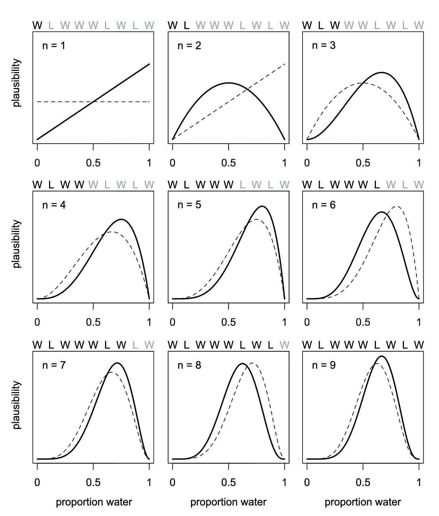
W L W W W L W L W (W indicates water and L indicates land.)
Procedure 2.2 : Designing a simple Bayesian model
“Designing a simple Bayesian model benefits from a design loop with three steps.
- Data story: Motivate the model by narrating how the data might arise.
- Update: Educate your model by feeding it the data.
- Evaluate: All statistical models require supervision, leading to model revision.” (McElreath, 2020, p. 28) (pdf)
2.2.1.1 A Data Story
“Bayesian data analysis usually means producing a story for how the data came to be. This story may be descriptive, specifying associations that can be used to predict outcomes, given observations. Or it may be causal, a theory of how some events produce other events.” (McElreath, 2020, p. 28) (pdf)
“… all data stories are complete, in the sense that they are sufficient for specifying an algorithm for simulating new data.” (McElreath, 2020, p. 28) (pdf)
Data story for our case
“The data story in this case is simply a restatement of the sampling process:
- The true proportion of water covering the globe is \(p\).
- A single toss of the globe has a probability p of producing a water (\(W\)) observation. It has a probability \(1 − p\) of producing a land (\(L\)) observation.
- Each toss of the globe is independent of the others.” (McElreath, 2020, p. 29) (pdf)
Data stories are important:
“Most data stories are much more specific than are the verbal hypotheses that inspire data collection. Hypotheses can be vague, such as”it’s more likely to rain on warm days.” When you are forced to consider sampling and measurement and make a precise statement of how temperature predicts rain, many stories and resulting models will be consistent with the same vague hypothesis. Resolving that ambiguity often leads to important realizations and model revisions, before any model is fit to data.” (McElreath, 2020, p. 29) (pdf)
2.2.1.2 Bayesian Updating
“Each possible proportion may be more or less plausible, given the evidence. A Bayesian model begins with one set of plausibilities assigned to each of these possibilities. These are the prior plausibilities. Then it updates them in light of the data, to produce the posterior plausibilities. This updating process is a kind of learning, called Bayesian updating.” (McElreath, 2020, p. 29) (pdf)
How a Bayesian model learns
Graph 2.1 helps to understand the Bayesian updating process. In R Code 2.4 we will learn how to write R code to reproduce the book’s figure as Graph 2.2. To inspect the different steps of the updating process is essential to understand Bayesian statistics!
2.2.1.3 Evaluate
Keep in mind two cautious principles:
“First, the model’s certainty is no guarantee that the model is a good one.” (McElreath, 2020, p. 31) (pdf) “Second, it is important to supervise and critique your model’s work.” (McElreath, 2020, p. 31) (pdf)
Test Before You Est(imate)
In the planned third version of the book McElreath wants to include from the beginning the evaluation part of the process. It is mentioned in the book already in this chapter 2 but without practical implementation and code examples. But we can find some remarks in his Statistical Rethinking Videos 2023b 37:40.
I will not go into details here, because my focus is on the second edition. But I will add as a kind of summary general advises for the testing procedure:
: Model evaluation
- Code a generative simulation
- Code an estimator
- Test the estimator with (1)
- where the answer is known
- at extreme values
- explore different sampling designs
- develop generally an intuition for sampling and estimation
Here are some references to get some ideas of the necessary R Code:
R Code snippets for testing procedure
- Simulating globe tossing: Statistical Rethinking 2023 - Lecture 02, Slide 54
- Simulate the experiment arbitrary times for any particular proportion: This is a way to explore the design of an experiment as well as debug the code. (Video 2023-02 39:55)
- Test the simulation at extreme values: R code snippets at Slide 57.
2.2.2 TIDYVERSE
Instead of vectors the tidyverse approach works best with data frames respectively tibbles. So let’s save the globe-tossing data W L W W W L W L W into a tibble:
R Code 2.2 : Save globe tossing data into a tibble
2.2.2.1 A Data Story
2.2.2.2 Bayesian Updating
For the updating process we need to add to the data the cumulative number of trials, n_trials, and the cumulative number of successes, n_successes with toss == "w".
R Code 2.3 : Bayesian updating preparation
The program code for reproducing the Figure 2.5 of the book (here in this document it is Graph 2.1) is pretty complex. I have to inspect the results line by line. At first I will give a short introduction what each line does. In the next steps I will explain each step more in detail and show the result of the corresponding lines of code.
Parameter \(k\) in lag() changed to \(default\)
R Code 2.4 : Bayesian updating: How a model learns
Code: How a Bayesian model learns
## (0) starting with tibble from the previous two code chunks #####
d <- tibble::tibble(toss = c("w", "l", "w", "w", "w", "l", "w", "l", "w")) |>
    dplyr::mutate(n_trials  = 1:9, n_success = cumsum(toss == "w"))

## (1) create tibble from all input combinations ################
sequence_length <- 50
d |>
  tidyr::expand_grid(p_water = seq(from = 0, to = 1,
                            length.out = sequence_length)) |>

## (2) group data by the `p-water` parameter ####################
  dplyr::group_by(p_water) |>

## (3) create columns filled with the value of the previous rows #####
  dplyr::mutate(lagged_n_trials  = dplyr::lag(n_trials, default = 1),
         lagged_n_success = dplyr::lag(n_success, default = 1)) |>

## (4) restore the original ungrouped data structure #######
  dplyr::ungroup() |>

## (5) calculate prior and likelihood & store values ######
  dplyr::mutate(prior      = ifelse(n_trials == 1, .5,
                             dbinom(x    = lagged_n_success,
                                    size = lagged_n_trials,
                                    prob = p_water)),
         likelihood = dbinom(x    = n_success,
                             size = n_trials,
                             prob = p_water),
         strip      = stringr::str_c("n = ", n_trials)) |>

## (6) normalize prior and likelihood ##########################
  dplyr::group_by(n_trials) |>
  dplyr::mutate(prior      = prior / sum(prior),
         likelihood = likelihood / sum(likelihood)) |>

  ## (7) plot the result ########################################
  ggplot2::ggplot(ggplot2::aes(x = p_water)) +
  ggplot2::geom_line(ggplot2::aes(y = prior), linetype = 2) +
  ggplot2::geom_line(ggplot2::aes(y = likelihood)) +
  ggplot2::scale_x_continuous("proportion water",
                     breaks = c(0, .5, 1)) +
  ggplot2::scale_y_continuous("plausibility", breaks = NULL) +
  ggplot2::theme(panel.grid = ggplot2::element_blank()) +
  ggplot2::facet_wrap(~ strip, scales = "free_y") +
ggplot2::theme_bw() 
2.2.2.2.1 Annotation (1): tidyr::expand_grid()
tidyr::expand_grid() creates a tibble from all combinations of inputs. Input are generalized vectors in contrast to tidyr::expand() that generates all combination of variables as well but needs as input a dataset. The range between 0 and 1 is divided into 50 part and then it generates all combinations by varying all columns from left to right. The first column is the slowest, the second is faster and so on.). It generates 450 data points (\(50 \times 9\) trials).
R Code 2.5 : Bayesian Update: Create tibble with all Input combinations
Code
#> # A tibble: 450 × 4
#>    toss  n_trials n_success p_water
#>    <chr>    <int>     <int>   <dbl>
#>  1 w            1         1  0
#>  2 w            1         1  0.0204
#>  3 w            1         1  0.0408
#>  4 w            1         1  0.0612
#>  5 w            1         1  0.0816
#>  6 w            1         1  0.102
#>  7 w            1         1  0.122
#>  8 w            1         1  0.143
#>  9 w            1         1  0.163
#> 10 w            1         1  0.184
#> # ℹ 440 more rows
2.2.2.2.2 Annotation (2): dplyr::group_by()
At first I did not understand the line group_by(p_water). Why has the data to be grouped when every row has a different value — as I have thought from a cursory inspection of the result? But it turned out that after 50 records the parameter p_water is repeating its value.
R Code 2.6 : Bayesian Updating: Lagged with grouping
Code
tbl1 <- tbl |>
  tidyr::expand_grid(p_water = seq(from = 0, to = 1,
                            length.out = sequence_length)) |>

  dplyr::group_by(p_water) |>
  dplyr::mutate(lagged_n_trials  = dplyr::lag(n_trials, default = 1),
         lagged_n_success = dplyr::lag(n_success, default = 1)) |>
  dplyr::ungroup() |>


  # add new column ID with row numbers
  # and relocate it to be the first column
  dplyr::mutate(ID = dplyr::row_number()) |>
  dplyr::relocate(ID, .before = toss)

# show 2 records from different groups
tbl1[c(1:2, 50:52, 100:102, 150:152), ]
#> # A tibble: 11 × 7
#> ID toss n_trials n_success p_water lagged_n_trials lagged_n_success
#> <int> <chr> <int> <int> <dbl> <int> <int>
#> 1 1 w 1 1 0 1 1
#> 2 2 w 1 1 0.0204 1 1
#> 3 50 w 1 1 1 1 1
#> 4 51 l 2 1 0 1 1
#> 5 52 l 2 1 0.0204 1 1
#> 6 100 l 2 1 1 1 1
#> 7 101 w 3 2 0 2 1
#> 8 102 w 3 2 0.0204 2 1
#> 9 150 w 3 2 1 2 1
#> 10 151 w 4 3 0 3 2
#> 11 152 w 4 3 0.0204 3 2I want to see the differences in detail. So I will provide also the ungrouped version.
R Code 2.7 : Bayesian Updating: Lagged without grouping
Code
tbl2 <- tbl |>
  tidyr::expand_grid(p_water = seq(from = 0, to = 1,
                            length.out = sequence_length)) |>

  dplyr::mutate(lagged_n_trials  = dplyr::lag(n_trials, default = 1),
         lagged_n_success = dplyr::lag(n_success, default = 1)) |>

  # add new column ID with row numbers and relocate it as first column
  dplyr::mutate(ID = dplyr::row_number()) |>
  dplyr::relocate(ID, .before = toss)

# show the same records without grouping
tbl2[c(1:2, 50:52, 100:102, 150:152), ]
#> # A tibble: 11 × 7
#> ID toss n_trials n_success p_water lagged_n_trials lagged_n_success
#> <int> <chr> <int> <int> <dbl> <int> <int>
#> 1 1 w 1 1 0 1 1
#> 2 2 w 1 1 0.0204 1 1
#> 3 50 w 1 1 1 1 1
#> 4 51 l 2 1 0 1 1
#> 5 52 l 2 1 0.0204 2 1
#> 6 100 l 2 1 1 2 1
#> 7 101 w 3 2 0 2 1
#> 8 102 w 3 2 0.0204 3 2
#> 9 150 w 3 2 1 3 2
#> 10 151 w 4 3 0 3 2
#> 11 152 w 4 3 0.0204 4 3It turned out that the two version differ after 51 records in the lagged variables. (Not after 50 as I would have assumed. Apparently this has to do with the lag() command because the first 51 records are identical. Beginning with row number 52 there are differences in the column lagged_n_trials and lagged_n_success. This pattern is repeated: Original version always changes after 100 records. The version without grouping changes after 50 rows starting with row 51.
2.2.2.2.3 Annotation (3): dplyr::lag()
The function dplyr::lag() finds the “previous” values in a vector (time series). This is useful for comparing values behind of the current values. See Compute lagged or leading values.
We need to get the immediately previous values for drawing the prior probabilities in the current graph (= dashed line or linetype = 2 in {ggplot2} parlance). In the relation with the posterior probabilities the difference form the prior possibility is always \(1\) (this is the option default = 1 in the dplyr::lag() function. This is now the correct explanation for the differences starting after rows 51 (and not 50).
2.2.2.2.4 Annotation (4): dplyr::ungroup()
This is just the reversion of the grouping command group_by(p_water).
2.2.2.2.5 Annotation (5): dbinom()
This is the core of the prior and likelihood calculation. It uses base::dbinom(), to calculate two alternative events. dbinom() is the R function for the binomial distribution, a distribution provided by the probability theory for “coin tossing” problems.
Exploring the dbinom() function
The distribution zoo is a nice resource to explore the shapes and properties of important Bayesian distributions. This interactive {shiny} app was developed by Ben Lambert and Fergus Cooper.
Choose “Discrete Univariate” as the “Category of Distribution” and then select as “Binomial” as the “Distribution Type”.
See also the two blog entries An Introduction to the Binomial Distribution and A Guide to dbinom, pbinom, qbinom, and rbinom in R of the Statology website.
The “d” in dbinom() stands for density. Functions named in this way almost always have corresponding partners that begin with “r” for random samples and that begin with “p” for cumulative probabilities. See for example the help file.
The results of each of the different calculation (prior and likelihood) are collected with dplyr::mutate() into two new generated columns.
There is no prior for the first trial, so it is assumed that it is 0.5. The formula for the binomial distribution uses for the prior the lagged-version whereas the likelihood uses the current version. These two lines provide the essential calculations: They match the 50 grid points as assumed water probabilities of every trial to their trial outcome (W or L) probabilities.
The last dplyr::mutate() command generates the \(strip\) variable consisting of the prefix \(n =\) followed by the counts of the number of trials. This will later provide the title for the the different facets of the plot.
To-do: Construct labelling specification for toss results
To get a better replication I would need to change the labels for the facets from n = n_trials to the appropriate string length of the results, e.g., for \(n = 3\) I would need \(W, L, W\).
This was not done by Kurz. I have tried it but didn’t succeed up to now (2023-10-25).
R Code 2.8 : Bayesian Updating: Calculating prior and likelihood
Code
#> # A tibble: 450 × 10
#>       ID toss  n_trials n_success p_water lagged_n_trials lagged_n_success prior
#>    <int> <chr>    <int>     <int>   <dbl>           <int>            <int> <dbl>
#>  1     1 w            1         1  0                    1                1   0.5
#>  2     2 w            1         1  0.0204               1                1   0.5
#>  3     3 w            1         1  0.0408               1                1   0.5
#>  4     4 w            1         1  0.0612               1                1   0.5
#>  5     5 w            1         1  0.0816               1                1   0.5
#>  6     6 w            1         1  0.102                1                1   0.5
#>  7     7 w            1         1  0.122                1                1   0.5
#>  8     8 w            1         1  0.143                1                1   0.5
#>  9     9 w            1         1  0.163                1                1   0.5
#> 10    10 w            1         1  0.184                1                1   0.5
#> # ℹ 440 more rows
#> # ℹ 2 more variables: likelihood <dbl>, strip <chr>
2.2.2.2.6 Annotation (6): Normalizing
The code lines in annotation 6 normalize the prior and the likelihood by grouping the data by n\_trials. Dividing every prior and likelihood values by their respective sum puts them both in a probability metric. This metric is important for the comparisons of different probabilities.
If you don’t normalize (i.e., divide the density by the sum of the density), their respective heights don’t match up with those in the text. Furthermore, it’s the normalization that makes them directly comparable. (Kurz in section Bayesian Updating of chapter 2)
R Code 2.9 : Bayesian Updating: Normalizing prior and likelihood
Code
#> # A tibble: 450 × 10
#> # Groups:   n_trials [9]
#>       ID toss  n_trials n_success p_water lagged_n_trials lagged_n_success prior
#>    <int> <chr>    <int>     <int>   <dbl>           <int>            <int> <dbl>
#>  1     1 w            1         1  0                    1                1  0.02
#>  2     2 w            1         1  0.0204               1                1  0.02
#>  3     3 w            1         1  0.0408               1                1  0.02
#>  4     4 w            1         1  0.0612               1                1  0.02
#>  5     5 w            1         1  0.0816               1                1  0.02
#>  6     6 w            1         1  0.102                1                1  0.02
#>  7     7 w            1         1  0.122                1                1  0.02
#>  8     8 w            1         1  0.143                1                1  0.02
#>  9     9 w            1         1  0.163                1                1  0.02
#> 10    10 w            1         1  0.184                1                1  0.02
#> # ℹ 440 more rows
#> # ℹ 2 more variables: likelihood <dbl>, strip <chr>
2.2.2.2.7 Annotation (7): Graphical demonstration of Bayesian updating
The remainder of the code prepares the plot by using the 50 grid points in the range from \(0\) to \(1\) as the x-axis; prior and likelihood as y-axis. To distinguish the prior from the likelihood it uses a dashed line for the prior (linetyp = 2) and a full line (default) for the likelihood. The x-axis has three breaks (\(0, 0.5, 1\)) whereas the y-axis has no break and no scale (scales = "free_y").
R Code 2.10 : Bayesian updating: Graphical demonstration
Code
tbl6 |>
  ggplot2::ggplot(ggplot2::aes(x = p_water)) +
  ggplot2::geom_line(ggplot2::aes(y = prior),
            linetype = 2) +
  ggplot2::geom_line(ggplot2::aes(y = likelihood)) +
  ggplot2::scale_x_continuous("proportion water", breaks = c(0, .5, 1)) +
  ggplot2::scale_y_continuous("plausibility", breaks = NULL) +
  ggplot2::theme(panel.grid = ggplot2::element_blank()) +
  ggplot2::theme_bw() +
ggplot2::facet_wrap(~ strip, scales = "free_y") 
2.3 Components of the Model
2.3.1 ORIGINAL
We observed three components of the model:
“(1) The number of ways each conjecture could produce an observation (2) The accumulated number of ways each conjecture could produce the entire data (3) The initial plausibility of each conjectured cause of the data” (McElreath, 2020, p. 32) (pdf)
2.3.1.1 Variables
“Variables are just symbols that can take on different values. In a scientific context, variables include things we wish to infer, such as proportions and rates, as well as things we might observe, the data. … Unobserved variables are usually called parameters.” (McElreath, 2020, p. 32) (pdf)
Take as example the globe tossing models: There are three variables: W and L (water or land) and the proportion of water and land p. We observe the events of water or land but we calculate (do not observe directly) the proportion of water and land. So p is a parameter as defined above.
2.3.1.2 Definitions
“Once we have the variables listed, we then have to define each of them. In defining each, we build a model that relates the variables to one another. Remember, the goal is to count all the ways the data could arise, given the assumptions. This means, as in the globe tossing model, that for each possible value of the unobserved variables, such as \(p\), we need to define the relative number of ways—the probability—that the values of each observed variable could arise. And then for each unobserved variable, we need to define the prior plausibility of each value it could take.” (McElreath, 2020, p. 33) (pdf)
Note 2.1 : Calculate the prior plausibility of the values of each observed variable in R
There are different functions in R that generate all combination of variables supplied by vectors, factors or data columns: base::expand.grid() or in the tidyverse tidyr::expand(), tidyr::expand_grid() and tidyr::crossing(). These functions can be used to calculate and generate the relative number of ways (= the probability) that the values of each observed variable could arise. We have seen a first demonstration in R Code 2.5. We will see many more examples in later sections and chapters.
2.3.1.2.1 Observed Variables
“For the count of water W and land L, we define how plausible any combination of W and L would be, for a specific value of p. This is very much like the marble counting we did earlier in the chapter. Each specific value of p corresponds to a specific plausibility of the data, as in Graph 2.3.
So that we don’t have to literally count, we can use a mathematical function that tells us the right plausibility. In conventional statistics, a distribution function assigned to an observed variable is usually called a likelihood. That term has special meaning in nonBayesian statistics, however.” (McElreath, 2020, p. 33) (pdf)
For our globe tossing procedure we use instead of counting a mathematical function to calculate the probability of all combinations.
“In this case, once we add our assumptions that (1) every toss is independent of the other tosses and (2) the probability of W is the same on every toss, probability theory provides a unique answer, known as the binomial distribution. This is the common”coin tossing” distribution.” (McElreath, 2020, p. 33) (pdf)
See also Section 2.2.2.2.5 for a resource to explore the binomial distribution.
R Code 2.11 : Likelihood for prob = 0.5 in the globe tossing example
The likelihood in the globe-tossing example (9 trials, 6 with W and 3 with L) is easily computed:
Code
## R code 2.2 ################
dbinom(6, size = 9, prob = 0.5)
#> [1] 0.1640625“Change the 0.5 to any other value, to see how the value changes.” (McElreath, 2020, p. 34) (pdf)
In this example it is assumed that the probability of W and L are equal distributed. We calculated how plausible the combination of \(6W\) and \(3L\) would be, for the specific value of \(p = 0.5\). The result is with \(16\%\) a pretty low probability.
To get a better idea what the best estimation of the probability is, we could vary systematically the \(p\) value and look for the maximum. A demonstration how this is done can be seen in R Code 2.12. It shows a maximum at \(prob = 0.7\).
2.3.1.2.2 Unobserved Variables
Even variables that are not observed (= parameters) we need to define them. In the globe-tossing model there is only one parameter (\(p\)), but most models have more than one unobserved variables.
Parameter & Prior
For every parameter we must provide a distribution of prior plausibility, its Prior Probability. This is also true when the number of trials is null (\(N = 0\)), e.g. even in the initial state of information we need a prior. (See R Code 2.4, where a flat prior was used.)
When you have a previous estimate, that can become the prior. As a result, each estimate (posterior probability) becomes then the prior for the next step (as you have seen in R Code 2.4).
“So where do priors come from? They are both engineering assumptions, chosen to help the machine learn, and scientific assumptions, chosen to reflect what we know about a phenomenon.” (McElreath, 2020, p. 35) (pdf)
“Within Bayesian data analysis in the natural and social sciences, the prior is considered to be just part of the model. As such it should be chosen, evaluated, and revised just like all of the other components of the model.” (McElreath, 2020, p. 35) (pdf)
“Beyond all of the above, there’s no law mandating we use only one prior. If you don’t have a strong argument for any particular prior, then try different ones. Because the prior is an assumption, it should be interrogated like other assumptions: by altering it and checking how sensitive inference is to the assumption.” (McElreath, 2020, p. 35) (pdf)
More on the difference between Bayesian and frequentist statistics?
Check out McElreath’s lecture, Understanding Bayesian statistics without frequentist language at Bayes@Lund2017 (20 April 2017).
2.3.1.3 A Model is Born
“The observed variables W and L are given relative counts through the binomial distribution.” (McElreath, 2020, p. 36) (pdf)
\[W∼Binomial(n,p) \space where\space N = W + L \tag{2.1}\]
“The above is just a convention for communicating the assumption that the relative counts of ways to realize \(W\) in \(N\) trials with probability \(p\) on each trial comes from the binomial distribution.” (McElreath, 2020, p. 36) (pdf)
Our binomial likelihood contains a parameter for an unobserved variable, p.
\[p∼Uniform(0,1) \tag{2.2}\]
The formula expresses the model assumption that the entire range of possible values for \(p\) are equally plausible.
###TIDYVERSE
Given a probability of .5, (e.g. equal probability to both events W and L) we use the dbinom() function to determine the likelihood of 6 out of 9 tosses coming out water in R Code 2.11.
McElreath suggests:
“Change the 0.5 to any other value, to see how the value changes.” (McElreath, 2020, p. 34) (pdf)
R Code 2.12 : Calculation likelihood with 10 different values of prob
Code
#> # A tibble: 11 × 2
#>     prob likelihood
#>    <dbl>      <dbl>
#>  1   0    0
#>  2   0.1  0.0000612
#>  3   0.2  0.00275
#>  4   0.3  0.0210
#>  5   0.4  0.0743
#>  6   0.5  0.164
#>  7   0.6  0.251
#>  8   0.7  0.267
#>  9   0.8  0.176
#> 10   0.9  0.0446
#> 11 1 0In the series of values you will notice several point:
- The values start with zero until a maximum of \(0.267\) and decline to zero again. The maximum is with \(prob = 0.7\), a proportion of \(W\) and \(L\) that is — as we know from our large world knowledge (knowledge outside the small world of the model) — already pretty near the real distribution of about \(0.71\). (see How Much of the Earth Is Covered by Water?)
- You see that the first
prob(\(0\)) and lastprob(\(1\)) values are both zero. From the result (6 \(W\) and 3 \(L\))probcannot be 0 or 1 because there a both \(W\) and \(L\) in the observed sample.
R Code 2.12 is my interpretation from the quote “Change the 0.5 to any other value, to see how the value changes.” Kurz has another interpretation when he draws a graph of 100 prob values from 0 to 1:
R Code 2.13 : Plot likelihood for 100 values of prob from \(0\) to \(1\), by steps of \(0.01\)
Code
tibble::tibble(prob = seq(from = 0, to = 1, by = .01)) |>
  ggplot2::ggplot(ggplot2::aes(x = prob, y = dbinom(x = 6, size = 9, prob = prob))) +
  ggplot2::geom_line() +
  ggplot2::labs(x = "probability",
       y = "binomial likelihood") +
  ggplot2::theme(panel.grid = ggplot2::element_blank()) +
  ggplot2::theme_bw()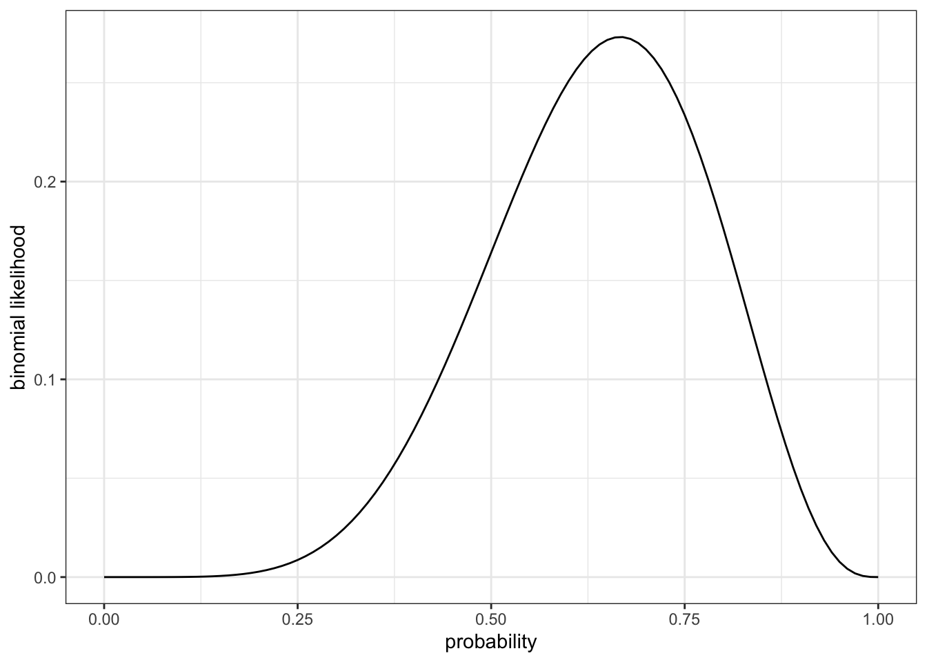
In contrast to \(p = 0.5\) with a probability of \(0.16\) the Graph 2.4 shows a maximum at about \(p = 0.7\) and a probability estimated from the graph of about \(0.26-0.28\). We will get more detailed data later in the book.
It is interesting to see that even the maximum probability is not very high. The reason is that there are many other configurations (distributions of \(W\)s and \(L\)s) to produce the result of \(6W\) and \(3L\). Even if all these other distributions have a small probability they “eat” all with their share from the maximum.
R Code 2.14 : Prior as a probability distribution for the parameter
“The prior is a probability distribution for the parameter. In general, for a uniform prior from \(a\) to \(b\), the probability of any point in the interval is \(1/(b − a)\). If you’re bothered by the fact that the probability of every value of \(p\) is \(1\), remember that every probability distribution must sum (integrate) to \(1\).” (McElreath, 2020, p. 35) (pdf)
Kurz demonstrates the truth of this quote with several \(b\) values while holding \(a\) constant:
#> # A tibble: 5 × 3
#>       a     b  prob
#>   <dbl> <dbl> <dbl>
#> 1     0   1   1
#> 2     0   1.5 0.667
#> 3     0   2   0.5
#> 4     0   3   0.333
#> 5     0   9   0.111
Verified with a plot Kurz divides the range of the \(b\) parameter (\(0-9\)) into 500 segments (parameter_space) and uses the dunif() distribution to calculate the probabilities for a uniform distribution:
Code
tibble::tibble(a = 0,
       b = c(1, 1.5, 2, 3, 9)) |>
  tidyr::expand_grid(parameter_space = seq(from = 0, to = 9, length.out = 500)) |>
  dplyr::mutate(prob = dunif(parameter_space, a, b),
         b    = stringr::str_c("b = ", b)) |>

  ggplot2::ggplot(ggplot2::aes(x = parameter_space, y = prob)) +
  ggplot2::geom_area() +
  ggplot2::scale_x_continuous(breaks = c(0, 1:3, 9)) +
  ggplot2::scale_y_continuous(breaks = c(0, 1/9, 1/3, 1/2, 2/3, 1),
                     labels = c("0", "1/9", "1/3", "1/2", "2/3", "1")) +
  ggplot2::theme(panel.grid.minor = ggplot2::element_blank(),
        panel.grid.major.x = ggplot2::element_blank()) +
  ggplot2::theme_bw() +
  ggplot2::facet_wrap(~ b, ncol = 5)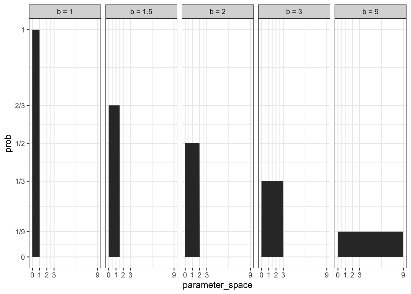
This figure demonstrates that the area in the whole parameter space is 1.0. It is a nice example how to calculate the probability mass (in contrast to the curve of the probability density).
2.4 Making the Model Go
“Once you have named all the variables and chosen definitions for each, a Bayesian model can update all of the prior distributions to their purely logical consequences: the ´r glossary(”posterior distribution”)`. For every unique combination of data, likelihood, parameters, and prior, there is a unique posterior distribution. This distribution contains the relative plausibility of different parameter values, conditional on the data and model. The posterior distribution takes the form of the probability of the parameters, conditional on the data.” (McElreath, 2020, p. 36) (pdf)
In the case of the globe-tossing model we can write:
\[ Pr(p|W, L) \tag{2.3}\]
This has to be interpreted as “the probability of each possible value of p, conditional on the specific \(W\) and \(L\) that we observed.”
2.4.1 Bayes’ Theorem
2.4.1.1 ORIGINAL
The Bayes’ theorem or Bayes’ rule gives Bayesian data analysis its name. What follows is a quick derivation of it. At first glance this might be too theoretical but after reading different books on Bayesian statistics I got the impression that it is not only important to know where the formula comes from but also what it stands for.
Theorem 2.1 : Bayes Theorem
“The joint probability of the data W and L and any particular value of p is:” (McElreath, 2020, p. 37) (pdf)
\[ Pr(W, L, p) = Pr(W, L \mid p) Pr(p) \tag{2.4}\]
“This just says that the probability of W, L and p is the product of Pr(W, L|p) and the prior probability Pr(p). This is like saying that the probability of rain and cold on the same day is equal to the probability of rain, when it’s cold, times the probability that it’s cold. This much is just definition. But it’s just as true that:” (McElreath, 2020, p. 37) (pdf)
\[ Pr(W, L, p) = Pr(p \mid W, L) Pr(W, L) \tag{2.5}\]
“All I’ve done is reverse which probability is conditional, on the right-hand side. It is still a true definition. It’s like saying that the probability of rain and cold on the same day is equal to the probability that it’s cold, when it’s raining, times the probability of rain.” (McElreath, 2020, p. 37) (pdf)
“Now since both right-hand sides above are equal to the same thing, \(Pr(W, L, p)\), they are also equal to one another:” (McElreath, 2020, p. 37) (pdf)
\[ \begin{align*} Pr(W, L \mid p) Pr(p) = Pr(p \mid W, L) Pr(W, L) \\ Pr(p\mid W, L) = \frac{Pr(W, L \mid p) Pr(p)}{Pr(W, L)} \end{align*} \tag{2.6}\]
“And this is Bayes’ theorem. It says that the probability of any particular value of \(p\), considering the data, is equal to the product of the relative plausibility of the data, conditional on \(p\), and the prior plausibility of \(p\), divided by this thing \(Pr(W, L)\), which I’ll call the average probability of the data.” (McElreath, 2020, p. 37) (pdf)
Expressed in words:
\[ Posterior = \frac{Probability\space of\space the\space data\space ✕\space Prior}{Average\space probability\space of\space the\space data} \tag{2.7}\]
Other names for the somewhat confusing average probability of the data:
- evidence
- average likelihood
- marginal likelihood
“The probability \(Pr(W, L)\) is literally the average probability of the data. Averaged over what? Averaged over the prior. It’s job is just to standardize the posterior, to ensure it sums (integrates) to one. In mathematical form:” (McElreath, 2020, p. 37) (pdf)
\[ PR(W, L) = E(Pr(W, L \mid p)) = \int Pr(W, L \mid p) Pr(p) dp \tag{2.8}\]
“The operator E means to take an expectation. Such averages are commonly called marginals in mathematical statistics, and so you may also see this same probability called a marginal likelihood. And the integral above just defines the proper way to compute the average over a continuous distribution of values, like the infinite possible values of \(p\).” (McElreath, 2020, p. 37) (pdf)
Key lesson about Bayes’ theorem
The posterior is proportional to the product of the prior and the probability of the data.
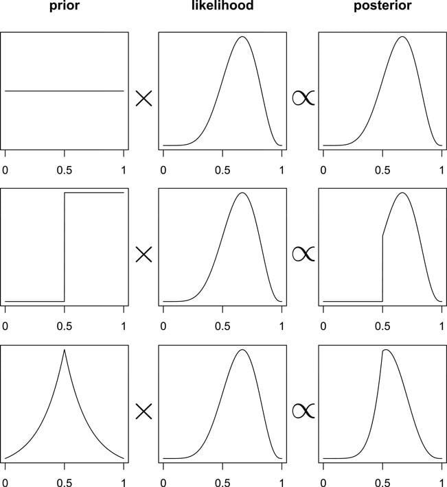
Graph 2.6 “illustrates the multiplicative interaction of a prior and a probability of data. On each row, a prior on the left is multiplied by the probability of data in the middle to produce a posterior on the right. The probability of data in each case is the same. The priors however vary. As a result, the posterior distributions vary.” (McElreath, 2020, p. 38) (pdf)
2.4.1.2 TIDYVERSE
For my understanding it is important to reproduce the Graph 2.6 graph with {tidyverse} R code as it is shown in the next section.
R Code 2.15 : The posterior distribution as a product of the prior distribution and likelihood
Code
sequence_length <- 1e3

d <-
  tibble::tibble(probability = seq(from = 0, to = 1,
                                   length.out = sequence_length)) |>
  tidyr::expand_grid(row = c("flat", "stepped", "Laplace"))  |>
  dplyr::arrange(row, probability) |>
  dplyr::mutate(
      prior = ifelse(row == "flat", 1,
              ifelse(row == "stepped", rep(0:1, each = sequence_length / 2),
                    exp(-abs(probability - 0.5) / .25) / ( 2 * 0.25))),
      likelihood = dbinom(x = 6, size = 9, prob = probability)) |>
  dplyr::group_by(row) |>
  dplyr::mutate(posterior = prior * likelihood / sum(prior * likelihood)) |>
  tidyr::pivot_longer(prior:posterior)  |>
  dplyr::ungroup() |>
  dplyr::mutate(
      name = forcats::fct(name, levels = c("prior", "likelihood", "posterior")),
      row  = forcats::fct(row, levels = c("flat", "stepped", "Laplace")))
In comparison to my very detailed code annotations of Graph 2.2 there are different lines of code, but generally there is nothing conceptually new: We use again expand_grid() to create a tibble of input combinations and create with mutate() two columns for prior and likelihood. We do not use the lag() functions as we calculate only for one prior and one likelihood. Kurz advises us that is “easier to just make each column of the plot separately. We can then use the elegant and powerful syntax from Thomas Lin Pedersen’s (2022) patchwork package to combine them.”
R Code 2.16 : Reproduction of book’s Graph 2.6
Code
p1 <-
  d |>
  dplyr::filter(row == "flat") |>
  ggplot2::ggplot(ggplot2::aes(x = probability, y = value)) +
  ggplot2::geom_line() +
  ggplot2::scale_x_continuous(NULL, breaks = NULL) +
  ggplot2::scale_y_continuous(NULL, breaks = NULL) +
  ggplot2::theme(panel.grid = ggplot2::element_blank()) +
  ggplot2::theme_bw() +
  ggplot2::facet_wrap(~ name, scales = "free_y")

p2 <-
  d |>
  dplyr::filter(row == "stepped") |>
  ggplot2::ggplot(ggplot2::aes(x = probability, y = value)) +
  ggplot2::geom_line() +
  ggplot2::scale_x_continuous(NULL, breaks = NULL) +
  ggplot2::scale_y_continuous(NULL, breaks = NULL) +
  ggplot2::theme(panel.grid = ggplot2::element_blank(),
        strip.background = ggplot2::element_blank(),
        strip.text = ggplot2::element_blank()) +
  ggplot2::theme_bw() +
  ggplot2::facet_wrap(~ name, scales = "free_y")

p3 <-
  d |>
  dplyr::filter(row == "Laplace") |>
  ggplot2::ggplot(ggplot2::aes(x = probability, y = value)) +
  ggplot2::geom_line() +
  ggplot2::scale_x_continuous(NULL, breaks = c(0, .5, 1)) +
  ggplot2::scale_y_continuous(NULL, breaks = NULL) +
  ggplot2::theme(panel.grid = ggplot2::element_blank(),
        strip.background = ggplot2::element_blank(),
        strip.text = ggplot2::element_blank()) +
  ggplot2::theme_bw() +
  ggplot2::facet_wrap(~ name, scales = "free_y")

# combine
library(patchwork)
p1 / p2 / p3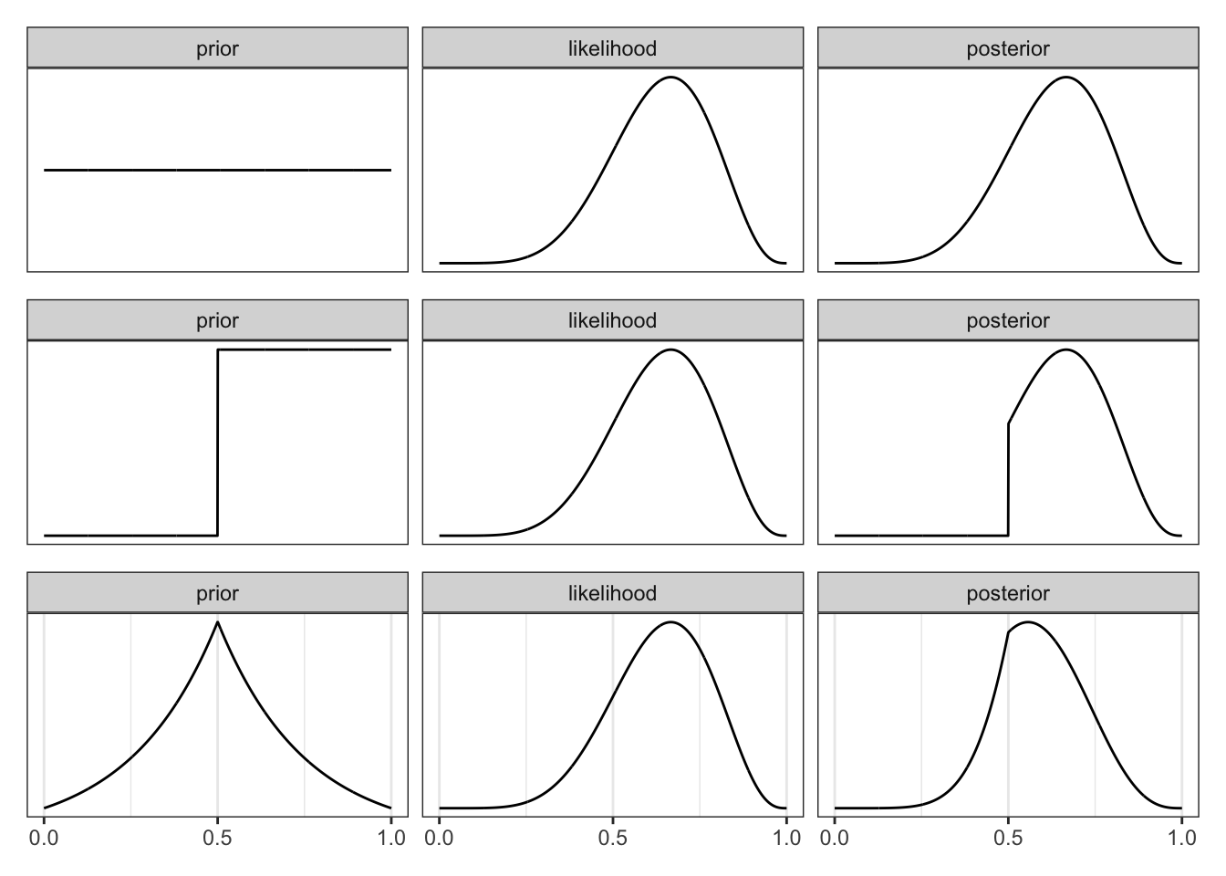
Graph 2.7 replicates Graph 2.6. It shows that the same likelihood with a different prior results in a different posterior.
2.4.2 Motors
2.4.2.1 ORIGINAL
The production of the posterior distribution is driven by a motor that conditions with it calculation the prior to the data. However, besides of simple and special restrictive models, often there is no formal mathematical solution. Therefore we need numerical techniques to approximate the mathematics.
Learning three different conditioning engines
“In this book, you’ll meet three different conditioning engines, numerical techniques for computing posterior distributions:
- Grid approximation
- Quadratic approximation
- Markov chain Monte Carlo (MCMC)
There are many other engines, and new ones are being invented all the time. But the three you’ll get to know here are common and widely useful. In addition, as you learn them, you’ll also learn principles that will help you understand other techniques.” (McElreath, 2020, p. 39) (pdf)
Fitting the model is part of the model
“… the details of fitting the model to data force us to recognize that our numerical technique influences our inferences. This is because different mistakes and compromises arise under different techniques. The same model fit to the same data using different techniques may produce different answers.” (McElreath, 2020, p. 39) (pdf)
2.4.2.2 TIDYVERSE (empty)
2.4.3 Grid approximation
2.4.3.1 ORIGINAL
“One of the simplest conditioning techniques is grid approximation. While most parameters are continuous, capable of taking on an infinite number of values, it turns out that we can achieve an excellent approximation of the continuous posterior distribution by considering only a finite grid of parameter values.” (McElreath, 2020, p. 39) (pdf)
Grid approximation is very useful as a pedagogical tool. But often it isn’t practical because it scales poorly, as the number of parameters increases.
Procedure 2.3 : Grid Approximation
“Here is the recipe:
- Define the grid. This means you decide how many points to use in estimating the posterior, and then you make a list of the parameter values on the grid.
- Compute the value of the prior at each parameter value on the grid.
- Compute the likelihood at each parameter value.
- Compute the unstandardized posterior at each parameter value, by multiplying the prior by the likelihood.
- Finally, standardize the posterior, by dividing each value by the sum of all values.” (McElreath, 2020, p. 40) (pdf)
I will outline in the globe tossing model the necessary steps for grid approximation. In addition to the 5 and 20 points approximation I will add 100 and 1000 points to see how the inferences changes with higher values.
R Code 2.17 : 6 Steps for Grid Approximation for the Globe Tossing Model
Code
## R code 2.3  adapted #########################

# 1. define grid
p_grid5 <- seq(from = 0, to = 1, length.out = 5)
p_grid20 <- seq(from = 0, to = 1, length.out = 20)
p_grid100 <- seq(from = 0, to = 1, length.out = 100)
p_grid1000 <- seq(from = 0, to = 1, length.out = 1000)

# 2. define prior
prior5 <- rep(1, 5)
prior20 <- rep(1, 20)
prior100 <- rep(1, 100)
prior1000 <- rep(1, 1000)

# 3. compute likelihood at each value in grid
likelihood5 <- dbinom(x = 6, size = 9, prob = p_grid5)
likelihood20 <- dbinom(x = 6, size = 9, prob = p_grid20)
likelihood100 <- dbinom(x = 6, size = 9, prob = p_grid100)
likelihood1000 <- dbinom(x = 6, size = 9, prob = p_grid1000)

# 4. compute product of likelihood and prior
unstd.posterior5 <- likelihood5 * prior5
unstd.posterior20 <- likelihood20 * prior20
unstd.posterior100 <- likelihood100 * prior100
unstd.posterior1000 <- likelihood1000 * prior1000

# 5. standardize the posterior, so it sums to 1
posterior5 <- unstd.posterior5 / sum(unstd.posterior5)
posterior20 <- unstd.posterior20 / sum(unstd.posterior20)
posterior100 <- unstd.posterior100 / sum(unstd.posterior100)
posterior1000 <- unstd.posterior1000 / sum(unstd.posterior1000)


# 6. display posterior distributions
op <- par(mfrow = c(2, 2))


## R code 2.4 ######################
## R code 2.4 for 5 points
plot(p_grid5, posterior5,
  type = "b",
  xlab = "probability of water", ylab = "posterior probability"
)
mtext('5 points with "prior = 1"')

## R code 2.4 for 20 points
plot(p_grid20, posterior20,
  type = "b",
  xlab = "probability of water", ylab = "posterior probability"
)
mtext('20 points with "prior = 1"')

## R code 2.4 for 100 points
plot(p_grid100, posterior100,
  type = "b",
  xlab = "probability of water", ylab = "posterior probability"
)
mtext('100 points with "prior = 1"')

## R code 2.4 for 1000 points
plot(p_grid1000, posterior1000,
  type = "b",
  xlab = "probability of water", ylab = "posterior probability"
)
mtext('1000 points with "prior = 1"')

par(op)
2.4.3.2 TIDYVERSE
Instead of just to replicate the globe-tossing steps with tidyverse code as in R Code 2.17 I will experiment with different priors to see their influences against the posterior distribution.
R Code 2.18 uses Kurz’ last code chunk in his grid approximation section. But I have adapted it to include the three uniform priors and to show also the (small) effect of 100 points grids.
Experiment: The effect of different priors and of different numbers of grid points.
The parameters for the calculated likelihood is based on the binomial distribution and is shaping the above plot:
-
x= number of water events \(W\) -
size= number of sample trials = number of observations -
prob= success probability on each trial = probability of \(W\) (water event)
I will only change prob and approximate the five different prior variants with 5, 20 and 100 points. I want to see how the effects of different priors on the posterior distribution by different number of events (grid points). The priors I will use are uniform priors of \(0.1\), \(0.5\) and \(0.9\), and the two suggestion by McElreath \(ifelse(p\_grid < 0.5, 0, 1)\) and \(exp(-5 * abs(p\_grid - 0.5))\).
R Code 2.18 : Globe tossing with different priors and grid points
Code
## R code 2.5 tidyverse integrated ################
# prepare the plot by producing the data

tib <-
tibble::tibble(n_points = c(5, 20, 100)) |>
  dplyr::mutate(p_grid = purrr::map(n_points, ~seq(from = 0, to = 1,
                                            length.out = .))) |>
  tidyr::unnest(p_grid) |>
  tidyr::expand_grid(priors = c("0.1",
                         "0.5",
                         "0.9",
                         "ifelse(p_grid < 0.5, 0, 1)",
                         "exp(-5 * abs(p_grid - 0.5))")) |>
  dplyr::mutate(prior = dplyr::case_when(
    priors == "0.1" ~ 0.1,
    priors == "0.5" ~ 0.5,
    priors == "0.9" ~ 0.9,
    priors == "ifelse(p_grid < 0.5, 0, 1)" ~ ifelse(p_grid < 0.5, 0, 1),
    priors == "exp(-5 * abs(p_grid - 0.5))" ~ exp(-5 * abs(p_grid - 0.5))
  )) |>
  dplyr::mutate(likelihood = dbinom(6, size = 9, prob = p_grid)) |>
  dplyr::mutate(posterior = likelihood * prior / sum(likelihood * prior)) |>
  dplyr::mutate(n_points = stringr::str_c("# points = ", n_points),
         priors   = stringr::str_c("prior = ", priors)) |>

  # plot the data
  ggplot2::ggplot(ggplot2::aes(x = p_grid, y = posterior)) +
  ggplot2::geom_line() +
  ggplot2::geom_point() +
  ggplot2::labs(x = "probability of water",
       y = "posterior probability") +
  ggplot2::theme(panel.grid = ggplot2::element_blank()) +
  ggplot2::theme_bw() +
  ggplot2::facet_grid(priors ~ n_points, scales = "free")
Inspecting the output we can draw some conclusions:
It does not matter what uniform prior probability is chosen in the range from 0 to 1, if the probability of \(W\) is greater than zero and — and by definition of the binomial function — equal for all events (grid points). This does not only conform to values but also for functions that generates values.
The only outlier in this sequence of different priors is the exponential function. But even this prior will finally give way if the number of observed events (approaching the real probability of 0.71) rises.
I will demonstrate this with 10000 samples and a W:L proportion of 7:3.
R Code 2.19 : Diminishing effect of the prior with rising amout of data
Code
d <-
    # 1.  define grid
    tibble::tibble(p_grid = seq(from = 0, to = 1, length.out = 100),
    # 2. define prior
           prior  = 1) |>
    # 3. compute likelihood at each value in grid
    dplyr::mutate(likelihood = dbinom(6, size = 9, prob = p_grid)) |>
    # 4. compute product of likelihood and prior
    dplyr::mutate(unstd_posterior = likelihood * prior) |>
    # 5. standardize the posterior, so it sums to 1
    dplyr::mutate(posterior = unstd_posterior / sum(unstd_posterior))

d |>
  ggplot2::ggplot(ggplot2::aes(x = p_grid, y = posterior)) +
  ggplot2::geom_point() +
  ggplot2::geom_line() +
  ggplot2::labs(title = "100 point grid approximation of 10000 samples with prior
       of exp(-5 * abs(p_grid - 0.5)) and a proportion of W:L = 7:3.",
       x = "probability of water",
       y = "posterior probability") +
  ggplot2::theme(panel.grid = ggplot2::element_blank()) +
  ggplot2::theme_bw()
In this example the maximum of probability is already 0.68! We can say that with every chosen prior we will get finally the correct result!.
But the choice of the prior is still important as it determines how many Bayesian updates we need to get the right result. If we have an awkward prior and not the appropriate size of the sample we will get a posterior distribution showing us a wrong maximum of probability. In that case the process of approximation has not reached a state where the probability maximum is near the correct result. The problem is: Most time we do not know the correct solution and can’t therefore decide if we have had enough Bayesian updates.
2.4.4 Quadratic Approximation
Grid approximation is very costly.
“The reason is that the number of unique values to consider in the grid grows rapidly as the number of parameters in your model increases. For the single-parameter globe tossing model, it’s no problem to compute a grid of 100 or 1000 values. But for two parameters approximated by 100 values each, that’s already 100^2 = 10,000 values to compute. For 10 parameters, the grid becomes many billions of values. These days, it’s routine to have models with hundreds or thousands of parameters.” ” (McElreath, 2020, p. 41f) (pdf)
Even grid approximation strategy scales poorly with model complexity it is very valuable for pedagogical reason. The two other strategies (Quadratic approximation and MCMC Methods) are better understood after examining in detail how grid approximation works.
2.4.4.1 ORIGINAL
2.4.4.1.1 Concept
“Under quite general conditions, the region near the peak of the posterior distribution will be nearly Gaussian—or”normal”—in shape. This means the posterior distribution can be usefully approximated by a Gaussian distribution. A Gaussian distribution is convenient, because it can be completely described by only two numbers: the location of its center (mean) and its spread (variance).
A Gaussian approximation is called “quadratic approximation” because the logarithm of a Gaussian distribution forms a parabola. And a parabola is a quadratic function. So this approximation essentially represents any log-posterior with a parabola.” (McElreath, 2020, p. 42) (pdf)
Procedure 2.4 : Quadratic Approximation
- Find the posterior mode with some optimization algorithm. The procedure does not know where the peak is but it knows the slope under its feet.
- Estimate the curvature near the peak to calculate a quadratic approximation. This computation is done by some numerical technique.
2.4.4.1.2 Computing the quadratic approximation
To compute the quadratic approximation for the globe tossing data, we’ll use a tool in the {rethinking} package: rethinking::quap().
R Code 2.20 : Quadratic approximation of the globe tossing data
Code
#>        mean        sd      5.5%     94.5%
#> p 0.6666667 0.1571338 0.4155366 0.9177968
“You can read this kind of approximation like: Assuming the posterior is Gaussian, it is maximized at \(0.67\), and its standard deviation is \(0.16\).” (McElreath, 2020, p. 43) (pdf)
Sometimes the quap() functions returns an error
If the quap() function does not compile because of an error, just try rendering the function or file again. The reason for the error? The function has chosen randomly a bad starting point for the approximation. (Later we will learn how to set start values to prevent such errors.)
Procedure 2.5 : Usage of rethinking::quap()
-
rethinking::quap()needs a formula, e.g., a list of data provided throughbase::alist(). -
alist()handles its arguments as if they described function arguments. So the values are not evaluated, and tagged arguments with no value are allowed. It is most often used in conjunction withbase::formals(). - The function
rethinking::precispresents a brief summary of the quadratic approximation.
- mean: It shows the posterior mean value of \(p = 0.67\). This is the peak of the posterior distribution.
- sd: The curvature is labeled “sd” This stands for standard deviation. This value is the standard deviation of the posterior distribution.
- 5.5% and 94.5%: These two values are the percentile intervals which will explained in Chapter 3.
2.4.4.1.3 Computing analytical solution
We want to compare the quadratic approximation with the analytic calculation.
“I’ll use the analytical approach here, which uses dbeta. I won’t explain this calculation, but it ensures that we have exactly the right answer. You can find an explanation and derivation of it in just about any mathematical textbook on Bayesian inference.” (McElreath, 2020, p. 43) (pdf)
R Code 2.21 : Comparing quadratic approximation with analytic calculation using dbeta()
Code
“The
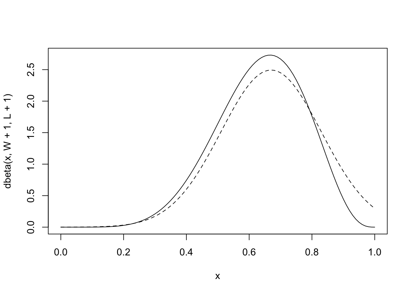
bluesolid line curve is the analytical posterior and theblackdashed curve is the quadratic approximation. Theblacksolid curve does alright on its left side, but looks pretty bad on its right side. It even assigns positive probability to \(p = 1\), which we know is impossible, since we saw at least one land sample” (McElreath, 2020, p. 43) (pdf)
2.4.4.2 TIDYVERSE
In the book the calculation is only done for \(n = 9\) but McElreath also display the graphs for \(n = 18\) and \(n = 36\) with the same proportion of W and L. Kurz shows how this is done and results into Figure 2.8 in the book.
R Code 2.22 : Quadratic approximation showing the effect of different sample size
Code
### quap() with 9 sample size #################################
globe_qa_9 <- rethinking::quap(
  alist(
    W ~ dbinom(W + L, p), # binomial likelihood
    p ~ dunif(0, 1) # uniform prior
  ),
  data = list(W = 6, L = 3)
)

# display summary of quadratic approximation
rethinking::precis(globe_qa_9)

### quap() with 18 sample size ###################################
globe_qa_18 <- rethinking::quap(
  alist(
    W ~ dbinom(W + L, p), # binomial likelihood
    p ~ dunif(0, 1) # uniform prior
  ),
  data = list(W = 12, L = 6)
)

# display summary of quadratic approximation
rethinking::precis(globe_qa_18)

### quap() with 36 sample size ###################################
globe_qa_36 <- rethinking::quap(
  alist(
    W ~ dbinom(W + L, p), # binomial likelihood
    p ~ dunif(0, 1) # uniform prior
  ),
  data = list(W = 24, L = 12)
)

# display summary of quadratic approximation
rethinking::precis(globe_qa_36)
#> mean sd 5.5% 94.5%
#> p 0.6666665 0.1571338 0.4155363 0.9177967
#> mean sd 5.5% 94.5%
#> p 0.6666663 0.1111104 0.4890903 0.8442422
#> mean sd 5.5% 94.5%
#> p 0.666667 0.07856685 0.541102 0.792232The results above displays values for sample size \(n = 9\) (top), \(n = 18\) (middle) and \(n = 36\) bottom. You can see that as the amount of data increases
- the mean approximates the real value
- the standard deviation and the percentile intervals gets smaller.
“As the amount of data increases, … the quadratic approximation gets better.” (McElreath, 2020, p. 43) (pdf)
“This phenomenon, where the quadratic approximation improves with the amount of data, is very common. It’s one of the reasons that so many classical statistical procedures are nervous about small samples: Those procedures use quadratic (or other) approximations that are only known to be safe with infinite data. Often, these approximations are useful with less than infinite data, obviously. But the rate of improvement as sample size increases varies greatly depending upon the details. In some models, the quadratic approximation can remain terrible even with thousands of samples.” (McElreath, 2020, p. 44) (pdf)
Graph 2.11 demonstrate that with more data the curve gets smaller and higher, signifying that the model gets more secure about the probability.
R Code 2.23 : Accuracy of the quadratic approximation with different sample sizes
Code
n_grid <- 100

# wrangle
tibble::tibble(w = c(6, 12, 24),
       n = c(9, 18, 36),
       s = c(.16, .11, .08)) |>
  tidyr::expand_grid(p_grid = seq(from = 0, to = 1, length.out = n_grid)) |>
  dplyr::mutate(prior = 1,
         m     = .67)  |>
  dplyr::mutate(likelihood = dbinom(w, size = n, prob = p_grid)) |>
  dplyr::mutate(unstd_grid_posterior = likelihood * prior,
         unstd_quad_posterior = dnorm(p_grid, m, s)) |>
  dplyr::group_by(w) |>
  dplyr::mutate(grid_posterior = unstd_grid_posterior / sum(unstd_grid_posterior),
         quad_posterior = unstd_quad_posterior / sum(unstd_quad_posterior),
         n              = stringr::str_c("n = ", n)) |>
 dplyr::mutate(n = forcats::fct(n, levels = c("n = 9", "n = 18", "n = 36"))) |>

  # plot
  ggplot2::ggplot(ggplot2::aes(x = p_grid)) +
  ggplot2::geom_line(ggplot2::aes(y = grid_posterior)) +
  ggplot2::geom_line(ggplot2::aes(y = quad_posterior),
            color = "grey50") +
  ggplot2::labs(x = "proportion water",
       y = "density") +
  ggplot2::theme(panel.grid = ggplot2::element_blank()) +
  ggplot2::theme_bw() +
  ggplot2::facet_wrap(~ n, scales = "free")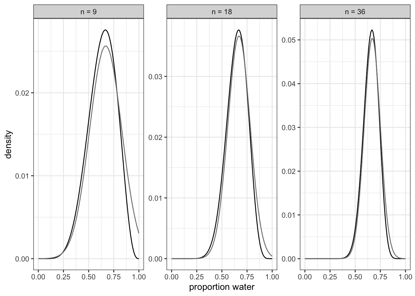
Textbooks highlighting MLE for GLMs
Kurz refers to three textbooks that highlight the maximum likelihood estimate (MLE) for the generalized linear model (GLM).
- Agresti. (2015). Foundations of Linear and Generalized Linear Models. Wiley.
- Dobson, A. J., & Barnett, A. G. (2018). An Introduction to Generalized Linear Models (4th ed.). Chapman and Hall/CRC.
- Dunn, P. K., & Smyth, G. K. (2018). Generalized Linear Models With Examples in R (1st ed. 2018 Edition). Springer.
(Agresti 2015; Dobson and Barnett 2018; Dunn and Smyth 2018)
Maximum Likelihood Estimation (MLE)
“The quadratic approximation, either with a uniform prior or with a lot of data, is often equivalent to a maximum likelihood estimate (MLE) and its standard error. The MLE is a very common non-Bayesian parameter estimate. This correspondence between a Bayesian approximation and a common non-Bayesian estimator is both a blessing and a curse. It is a blessing, because it allows us to re-interpret a wide range of published non-Bayesian model fits in Bayesian terms. It is a curse, because maximum likelihood estimates have some curious drawbacks, and the quadratic approximation can share them.” (McElreath, 2020, p. 44) (pdf)
2.4.5 Markov Chain Monte Carlo (MCMC)
2.4.5.1 ORIGINAL
“There are lots of important model types, like multilevel (mixed-effects) models, for which neither grid approximation nor quadratic approximation is always satisfactory.” (McElreath, 2020, p. 45) (pdf)
“As a result, various counterintuitive model fitting techniques have arisen. The most popular of these is Markov chain Monte Carlo (MCMC), which is a family of conditioning engines capable of handling highly complex models. It is fair to say that MCMC is largely responsible for the insurgence of Bayesian data analysis that began in the 1990s. While MCMC is older than the 1990s, affordable computer power is not, so we must also thank the engineers.” (McElreath, 2020, p. 45) (pdf)
“The conceptual challenge with MCMC lies in its highly non-obvious strategy. Instead of attempting to compute or approximate the posterior distribution directly, MCMC techniques merely draw samples from the posterior. You end up with a collection of parameter values, and the frequencies of these values correspond to the posterior plausibilities. You can then build a picture of the posterior from the histogram of these samples.” (McElreath, 2020, p. 45) (pdf)
The understanding of this not intuitive technique is postponed to ?sec-chap09. What follows is just a demonstration of the technique.
R Code 2.24 : Demo of the Markov Chain Monte Carlo (MCMC) method
Code
## R code 2.8 #######################
n_samples <- 1000
p <- rep(NA, n_samples)
p[1] <- 0.5
W <- 6
L <- 3
for (i in 2:n_samples) {
  p_new <- rnorm(1, p[i - 1], 0.1)
  if (p_new < 0) p_new <- abs(p_new)
  if (p_new > 1) p_new <- 2 - p_new
  q0 <- dbinom(W, W + L, p[i - 1])
  q1 <- dbinom(W, W + L, p_new)
  p[i] <- ifelse(runif(1) < q1 / q0, p_new, p[i - 1])
}

## R code 2.9 #######################
rethinking::dens(p, xlim = c(0, 1))
curve(dbeta(x, W + 1, L + 1), lty = 2, add = TRUE)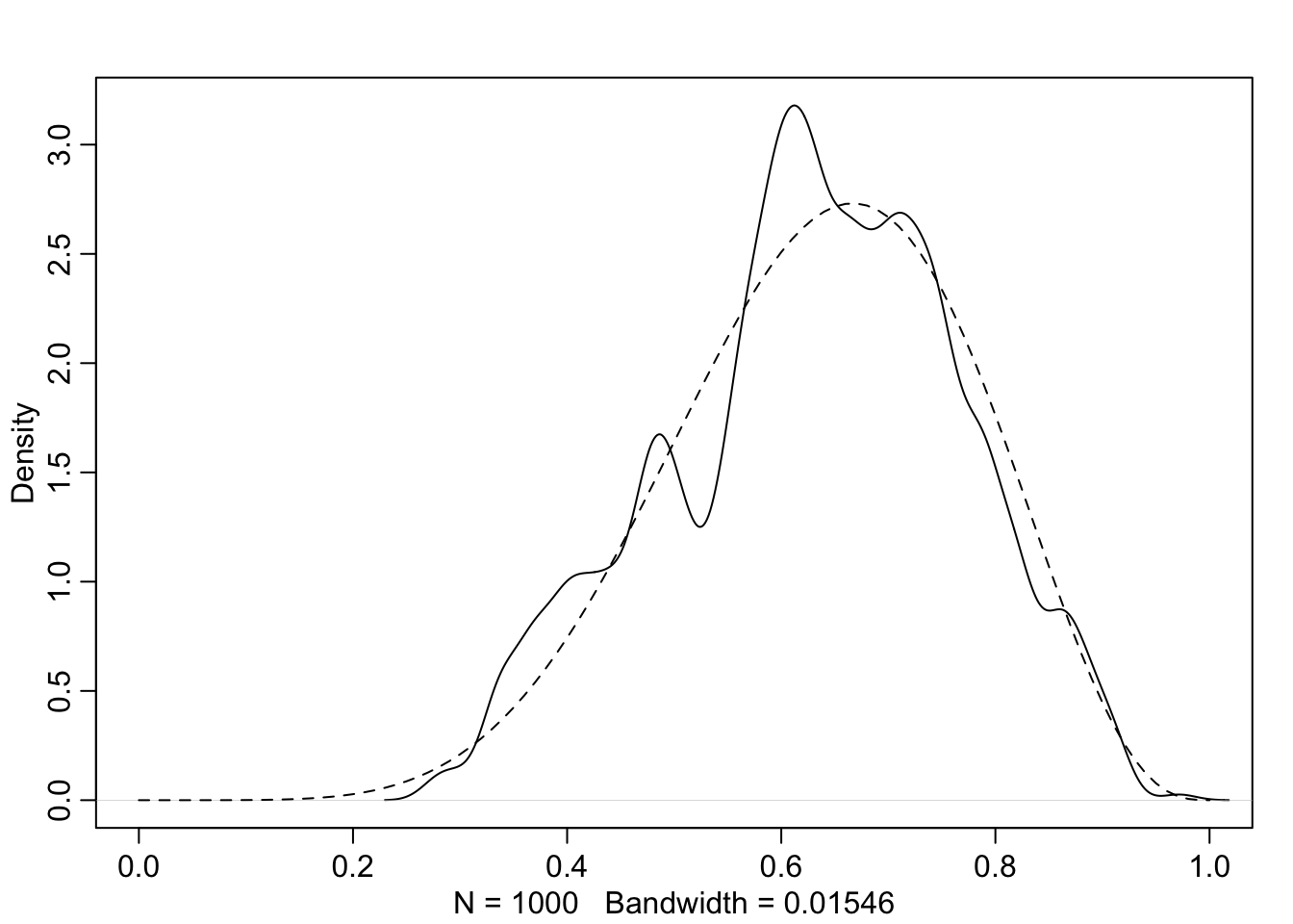
It’s weird. But it works. The metropolis algorithm used in #cnj-fig-demo-mcmc-rethinking is explained in ?sec-chap09.
2.4.5.2 TIDYVERSE
The {brms} package uses a version of MCMC to fit Bayesian models. brms stands for Bayesian Regression Models using Stan.
The main goals of the Kurz’ version is to highlight the {brms} package. Therefore we will use it instead just replicating the {rethinking}-version of MCMC.
If you haven’t already installed {brms}, you can find instructions on how to do on GitHub or on the corresponding website.)
As an exercise we will re-fit the model with \(W = 24\) and \(n = 36\) of R Code 2.22 and R Code 2.20.
{brms} and {rethinking} are conflicting packages
Preventing code conflicts
{brms} and {rethinking} are packages designed for similar purposes and therefore overlap in some of their function names. If you have loaded {rethinking} then you need to detach the package before loading {brms}. This is not necessary in my case, because I haven’t used the library() command.
To learn more on the topic, see this R-bloggers post. (This remark comes from section 4.3.1 of the Kurz version).
First compiling
Be patient when you render the following chunk the first time. It need some time. Furthermore it results in a very long processing message under the compiled chunk. Again this happens only the first time because the result is stored in the “fits” folder which you have to create before running the chunk.
To resume the necessary preparing steps I collected all to dos in a procedure callout:
Procedure 2.6 : Steps to use {brms} the first time
- Prevent code conflicts as explained in the previous watch-out callout.
- Download the {brms} package
- Load the package with
library()or use the package name followed by a double colon immediately before the function - Create a folder in the working directory of your project. The following code chunks suggest “fits” as folder name. If you are using another name then you have to change the scripts accordingly.
- Render the script and be patient especially the first time you ar compiling the script.
R Code 2.25 : Demonstration of the brm() function of the {brms} package.
Code
#>  Family: binomial
#>   Links: mu = identity
#> Formula: w | trials(36) ~ 0 + Intercept
#>    Data: list(w = 24) (Number of observations: 1)
#>   Draws: 4 chains, each with iter = 2000; warmup = 1000; thin = 1;
#>          total post-warmup draws = 4000
#>
#> Population-Level Effects:
#>           Estimate Est.Error l-95% CI u-95% CI Rhat Bulk_ESS Tail_ESS
#> Intercept     0.66      0.08     0.50     0.80 1.00     1537     1456
#>
#> Draws were sampled using sampling(NUTS). For each parameter, Bulk_ESS
#> and Tail_ESS are effective sample size measures, and Rhat is the potential
#> scale reduction factor on split chains (at convergence, Rhat = 1).
A detailed explanation of the result is postponed to Example 4.11. Here I will just copy the notes by Kurz to get a first understanding and a starting point for further exploration in the following chapters.
For now, focus on the ‘Intercept’ line. As we’ll also learn in Chapter 4, the intercept of a typical regression model with no predictors is the same as its mean. In the special case of a model using the binomial likelihood, the mean is the probability of a 1 in a given trial, \(\theta\).
Also, with {brms}, there are many ways to summarize the results of a model. The
brms::posterior_summary()function is an analogue torethinking::precis(). We will, however, need to useround()to reduce the output to a reasonable number of decimal places.
Code
brms::posterior_summary(b2.1) |>
  round(digits = 2)
#> Estimate Est.Error Q2.5 Q97.5
#> b_Intercept 0.66 0.08 0.50 0.80
#> lprior 0.00 0.00 0.00 0.00
#> lp__ -3.98 0.75 -6.03 -3.46The
b_Interceptrow is the probability. Don’t worry about the second line, for now. We’ll cover the details of {brms} model fitting in later chapters. To finish up, why not plot the results of our model and compare them with those fromrethinking::quap(), above? (See Graph 2.12)
Code
brms::as_draws_df(b2.1) |>
  dplyr::mutate(n = "n = 36") |>

  ggplot2::ggplot(ggplot2::aes(x = b_Intercept)) +
  ggplot2::geom_density(fill = "gray") +
  ggplot2::scale_x_continuous("proportion water", limits = c(0, 1)) +
  ggplot2::theme(panel.grid = ggplot2::element_blank()) +
  ggplot2::theme_bw() +
  ggplot2::facet_wrap(~ n)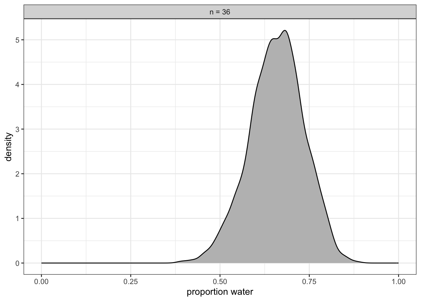
If you’re still confused, cool. This is just a preview. We’ll start walking through fitting models with brms in Chapter 4 and we’ll learn a lot about regression with the binomial likelihood in Chapter 11.
Using Bayesian Regression Models using Stan {brms}
- Website: Bayesian regression models using Stan
- Bürkner, P-C. (2017). brms: An R Package for Bayesian Multilevel Models Using Stan. Journal of Statistical Software, 80, 1–28. https://doi.org/10.18637/jss.v080.i01
- Bürkner, P-C. (2018). The R Journal: Advanced Bayesian Multilevel Modeling with the R Package brms. The R Journal, 10(1), 395–411. https://doi.org/10.32614/RJ-2018-017
- van de Schoot, R. (2019). BRMS. Series of tutorials how to run the brms package. Rens van de Schoot Webpage. https://www.rensvandeschoot.com/tutorials/brms/
- Nalborczyk, L. (2017). Appendix: An introduction to Bayesian multilevel models using brms | Understanding rumination as a form of inner speech. Retrieved October 31, 2023, from https://lnalborczyk.github.io/phd_thesis/appendix-brms.html
- Nalborczyk, L., Batailler, C., Loevenbruck, H., Vilain, A., & Bürkner, P.-C. (2017). An Introduction to Bayesian Multilevel Models Using brms: A Case Study of Gender Effects on Vowel Variability in Standard Indonesian. https://doi.org/10.17605/OSF.IO/DPZCB
- Ellis, A. (2021). Learn multilevel models: An Introduction to brms. https://awellis.github.io/learnmultilevelmodels/walkthrough-brms.html/
Bayesian Inference: Some Lessons to Draw
The following list summarizes differences between Bayesian and Non-Bayesian inference (frequentist statistics or “Frequentism”):
- No minimum sampling size: The minimum sampling size in Bayesian inference is one. You are going to update each data point at its time. For instance you got an estimate every time when you toss the globe and the estimate is updated. — Well, the sample size of one is not very informative but that is the power of Bayesian inference in not getting over confident. It is always accurately representing the relative confidence of plausability we should assign to each of the possible proportions.
- Shape embodies sample size: The shape of the posterior distribution embodies all the information that the sample has about the process of the proportions. Therefore you do not need to go back to the original dataset for new observations. Just take the posterior distribution and update it by multiplying the number of ways the new data could produce.
- No point estimates: The estimate is the whole distribution. It may be fine for communication purposes to talk about some summary points of the distribution like the mode and mean. But neither of these points is special as a point of estimate. When we do calculations we draw predictions from the whole distribution, never just from a point of it.
- No one true interval: Intervals are not important in Bayesian inference. They are merely summaries of the shape of the distribution. There is nothing special in any of these intervals because the endpoints of the intervals are not special. Nothing happens of the endpoints of the intervals because the interval is arbitrary. (The 95% in Non-Bayesian inference is essentially a dogma, a superstition. Even in Non-Bayesian statistics it is conceptualized as an arbitrary interval.)
2.5 Practice
2.5.1 Easy
2.5.1.1 2E1
Exercise 2E1: Which of the expressions below correspond to the statement: the probability of rain on Monday?
- \(Pr(rain)\)
- \(Pr(rain \mid Monday)\)
- \(Pr(Monday \mid rain)\)
- \(\frac{Pr(rain, Monday)}{Pr(Monday)}\)
My Solution
- and 4.
Watch out!
Originally I believed that only 2. is true. But both Erik Kusch and Jake Thompson also mentioned choice 4.
The explication by Erik Kusch convinced me:
- \(\frac{Pr(rain, Monday)}{Pr(Monday)}\) - reads as “the probability that is raining and a Monday, divided by the probability of it being a Monday” which is the same as “the probability of rain, given that it is Monday. This is simply just the Bayes theorem in action.”
2.5.1.2 2E2
Exercise 2E2: Which of the following statements corresponds to the expression: \(Pr(Monday|rain)\)?
- The probability of rain on Monday.
- The probability of rain, given that it is Monday.
- The probability that it is Monday, given that it is raining.
- The probability that it is Monday and that it is raining.
My Solution
2.5.1.3 2E3
Exercise 2E3: Which of the expressions below correspond to the statement: the probability that it is Monday, given that it is raining?
\((1) Pr(Monday|rain)\) \((2) Pr(rain|Monday)\) \((3) Pr(rain|Monday) Pr(Monday)\) \((4) \frac{Pr(rain|Monday) Pr(Monday)} {Pr(rain)}\) \((5) \frac{Pr(Monday|rain) Pr(rain)} {Pr(Monday)}\)
My Solution
- and 4.
Watch out!
Again I did not see/know that 4. the bayes’ theorem is also a correct solution. Again Kusch and Thompson had 1. and 4. as solution. This time Jake Thompson has a short explanation:
Answer option (1) is the standard notation for the conditional probability. Answer option (4) is equivalent, as this is Bayes’ Theorem.
2.5.1.4 2E4
Exercise 2E4: Does probability exist?
The Bayesian statistician Bruno de Finetti (1906–1985) began his 1973 book on probability theory with the declaration: “PROBABILITY DOES NOT EXIST.” The capitals appeared in the original, so I imagine de Finetti wanted us to shout this statement. What he meant is that probability is a device for describing uncertainty from the perspective of an observer with limited knowledge; it has no objective reality. Discuss the globe tossing example from the chapter, in light of this statement. What does it mean to say “the probability of water is 0.7”?
See (Finetti 2017; Galavotti 2008)
My Solution
As an observer we collected evidence (tossing the globe and collecting how many often our index finger hold the globe over water) that “the probability of water is 0.7”. But the word “probability” is only necessary as we have only limited knowledge. Beings with unlimited knowledge (e.g., “God”) would say “the earth has a proportion of 0.71:0.29 of water to land”. The word “probability” would not be necessary.
Watch out!
The answers to this question differ widely. One answer I like especially is from Jake Thompson:
The idea is that probability is only a subjective perception of the likelihood that something will happen. In the globe tossing example, the result will always be either “land” or “water” (i.e., 0 or 1). When we toss the globe, we don’t know what the result will be, but we know it will always be “land” or “water.” To express our uncertainty in the outcome, we use probability. Because we know that water is more likely than land, we may say that the probability of “water” is 0.7; however, we’ll never actually observe a result of 0.7 waters, or observe any probability. We will only ever observe the two results of “land” and “water.”
2.5.2 Middle
2.5.2.1 2M1
Exercise 2M1: Globe tossing model – Compute and plot the grid approximate posterior distribution for each of the following sets of observations
In each case, assume a uniform prior for \(p\).
- \(W, W, W\)
- \(W, W, W, L\)
- \(L, W, W, L, W, W, W\)
My Solution
R Code 2.26 : Compute and plot the grid approximate posterior distribution
Code
# prepare the plot by producing the data
df_2m1 <- tibble::tibble(grid_2m1 =
                 seq(from = 0, to = 1, length.out = 20)) |>
  dplyr::mutate(prior = 1,
                likelihood_1 = dbinom(3, size = 3, prob = grid_2m1),
                likelihood_2 = dbinom(3, size = 4, prob = grid_2m1),
                likelihood_3 = dbinom(5, size = 7, prob = grid_2m1),
                posterior_1 = likelihood_1 *
                  prior / sum(likelihood_1 * prior),
                posterior_2 = likelihood_2 *
                  prior / sum(likelihood_2 * prior),
                posterior_3 = likelihood_3 *
                  prior / sum(likelihood_3 * prior))


  # plot the data
  ggplot2::ggplot(data = df_2m1) +
    ggplot2::geom_line(ggplot2::aes(x = grid_2m1, y = posterior_1,
                                linetype = "(1) W, W, W")) +
    ggplot2::geom_line(ggplot2::aes(x = grid_2m1, y = posterior_2,
                                linetype = "(2) W, W, W, L")) +
    ggplot2::geom_line(ggplot2::aes(x = grid_2m1, y = posterior_3,
              linetype = "(3) L, W, W, L, W, W, W")) +
    ggplot2::scale_linetype_manual("Data:",
                        values = c("solid", "dashed", "dotted")) +
  ggplot2::labs(title =
  "Exercise 2M1: Grid approximation with uniform prior = 1, 20 points",
                x = "probability of water",
                y = "posterior probability") +
  ggplot2::theme(panel.grid = ggplot2::element_blank()) +
ggplot2::theme_bw() 
My original code was with 100 points and a uniform prior of 0.5. The shape of the curves conformed to both Kusch and Thompson, but the values of the y-axis were different. For a better comparison I chanced my code to the prior of 1 with 20 points.
BTW: The code from Thompson is very advanced. Obviously he is very experienced with R.
2.5.2.2 2M2
Exercise 2M2: Now assume a prior for \(p\) that is equal to zero when \(p < 0.5\) and is a positive constant when \(p ≥ 0.5\).
Again compute and plot the grid approximate posterior distribution for each of the sets of the observations
- \(W, W, W\)
- \(W, W, W, L\)
- \(L, W, W, L, W, W, W\)
My Solution
R Code 2.27 : Compute and plot the grid approximate posterior distribution
Code
# prepare the plot by producing the data
df_2m2 <- tibble::tibble(grid_2m2 =
                 seq(from = 0, to = 1, length.out = 20)) |>
  dplyr::mutate(prior = ifelse(grid_2m2 < 0.5, 0, 1)) |>
  dplyr::mutate(likelihood_1 = dbinom(3, size = 3, prob = grid_2m2),
                likelihood_2 = dbinom(3, size = 4, prob = grid_2m2),
                likelihood_3 = dbinom(5, size = 7, prob = grid_2m2),
                posterior_1 = likelihood_1 *
                  prior / sum(likelihood_1 * prior),
                posterior_2 = likelihood_2 *
                  prior / sum(likelihood_2 * prior),
                posterior_3 = likelihood_3 *
                  prior / sum(likelihood_3 * prior))


  # plot the data
  ggplot2::ggplot(data = df_2m2) +
    ggplot2::geom_line(ggplot2::aes(x = grid_2m2, y = posterior_1,
                                linetype = "(1) W, W, W")) +
    ggplot2::geom_line(ggplot2::aes(x = grid_2m2, y = posterior_2,
                                linetype = "(2) W, W, W, L")) +
    ggplot2::geom_line(ggplot2::aes(x = grid_2m2, y = posterior_3,
              linetype = "(3) L, W, W, L, W, W, W")) +
    ggplot2::scale_linetype_manual("Data:",
                        values = c("solid", "dashed", "dotted")) +
  ggplot2::labs(title =
  "Exercise 2M2: Grid approximation with 20 points a prior for p that is
equal to zero when p < 0.5 and is a positive constant when p ≥ 0.5",
                x = "probability of water",
                y = "posterior probability") +
  ggplot2::theme(panel.grid = ggplot2::element_blank()) +
ggplot2::theme_bw() 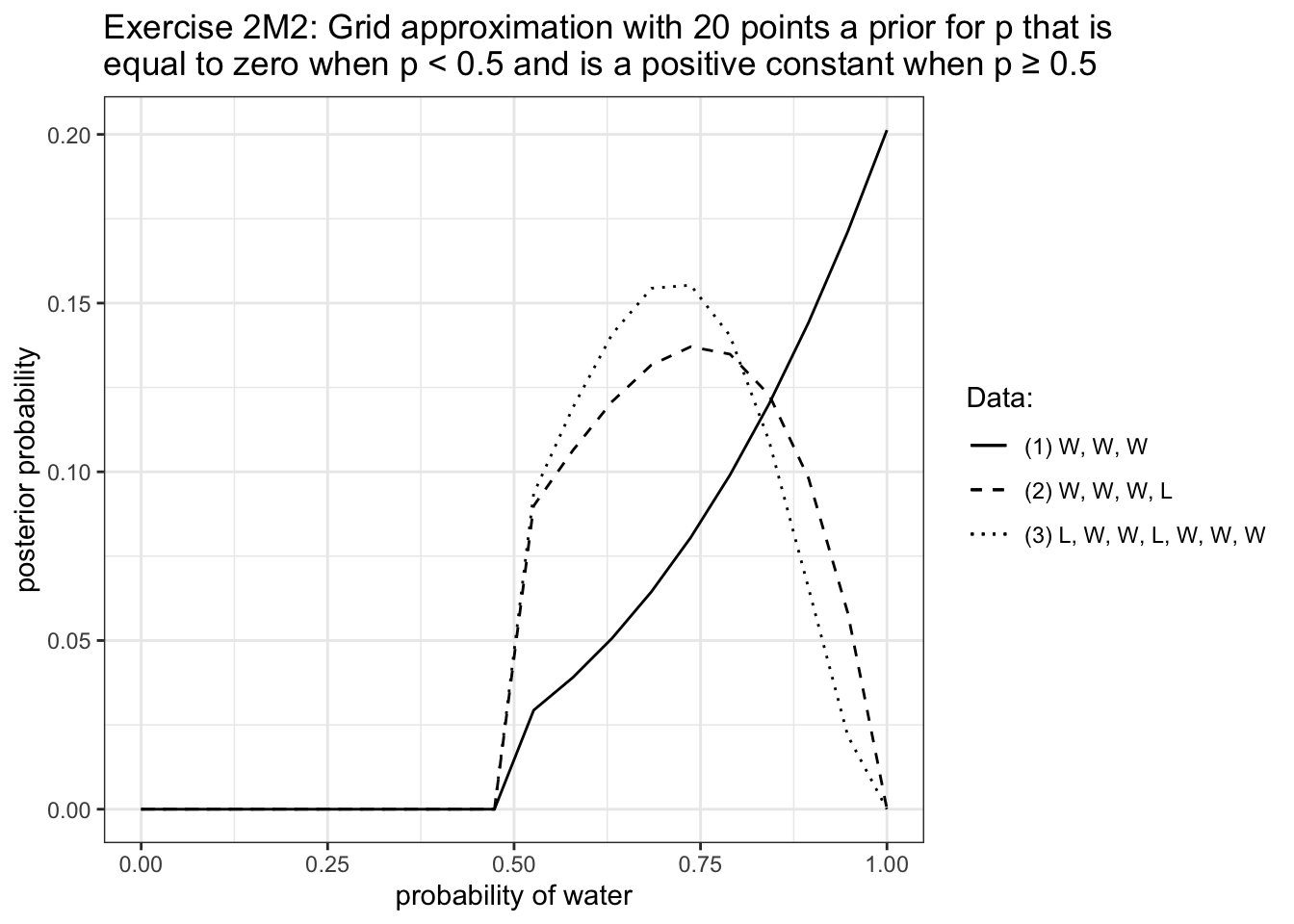
2.5.2.3 2M3
Exercise 2M3: Suppose there are two globes, one for Earth and one for Mars.
The Earth globe is \(70\%\) covered in water. The Mars globe is \(100\%\) land. Further suppose that one of these globes—you don’t know which—was tossed in the air and produced a “land” observation. Assume that each globe was equally likely to be tossed. Show that the posterior probability that the globe was the Earth, conditional on seeing “land” (\(Pr(Earth \mid land)\)), is \(0.23\).
My Solution
What do we know?
\[ \begin{align*} Pr(land \mid Earth) = 1 - 0.7 = 0.3 \\ Pr(land \mid Mars) = 1 \\ Pr(Earth) = Pr(Mars) = 0.5 \\ \text{Bayes’ theorem} = Pr(Earth \mid land) = \frac{Pr(land\mid Earth) Pr(Earth)}{Pr(land)} \\ Pr(land) \text{is the only value that is missing, can be caluclated by:} \\ Pr(land) = Pr(land \mid Earth)Pr(Earth) + Pr(land \mid Mars)Pr(Mars) \\ Pr(land) = 0.3 \times 0.5 + 1 \times 0.5 = 0.15 + 0.5 = 0.65 \\ \text{now we can plug in all values in Bayes’ theorem} \\ Pr(Earth \mid land) = \frac{0.3 \times 0.5 }{0.65} = 0.2307692 \end{align*} \tag{2.9}\]
Watch out!
I have to confess that I didn’t know the solution. I had to cheat and look at the solution of Aidan Marshall, Taras Svirskyi, Jake Thompson and Erik Kusch. All of them knew the correct answer!
My answers follows the solution of Erik Kusch. By this occasion I detected an error in my writing down the derivation of the Bayes’ theorem (Theorem 2.1). No surprise that I failed this exercise and all the others with the Bayes’ theorem as part of the solution ( 2E1 and 2E3).
2.5.2.4 2M4
Exercise 2M4: Suppose you have a deck with only three cards {#exercise-2m4}
Each card has two sides, and each side is either black or white. One card has two black sides. The second card has one black and one white side. The third card has two white sides.
Now suppose all three cards are placed in a bag and shuffled. Someone reaches into the bag and pulls out a card and places it flat on a table. A black side is shown facing up, but you don’t know the color of the side facing down.
Show that the probability that the other side is also black is 2/3. Use the counting method from section The Garden of Forking Data to approach this problem. This means counting up the ways that each card could produce the observed data (a black side facing up on the table).
My Solution
Watch out!
Again it seems that the way I tried to solve the exercise was wrong even if I got the correct result 1/3. I thought it would be enough to count the whole cards as ways and not the sides of the cards. Why? I thought that every card has just one side to make it visible for the observer.
So my solution counted the sample space as {B/B, B/W, W/W} and ways to produce a cards with a black side in front as {B/B, B/W}. \(\frac{Ways}{Sample Space} = \frac{2}{3}\)
But with the next example my method yields \(\frac{3}{4}\) whereas the solution of other people resulted in \(0.8\).
2.5.2.5 2M5
Exercise 2M5: Deck with four cards B/B, B/W, W/W, and B/B
Again suppose a card is drawn from the bag and a black side appears face up. Again calculate the probability that the other side is black.
My Solution
R Code 2.29 : Deck with four cards B/B, B/W, W/W, and B/B
2.5.2.6 2M6
Exercise 2M6: Card deck where cards with a black side are heavier
Imagine that black ink is heavy, and so cards with black sides are heavier than cards with white sides. As a result, it’s less likely that a card with black sides is pulled from the bag.
So again assume there are three cards: B/B, B/W, and W/W. After experimenting a number of times, you conclude that for every way to pull the B/B card from the bag, there are 2 ways to pull the B/W card and 3 ways to pull the W/W card.
Again suppose that a card is pulled and a black side appears face up. Show that the probability the other side is black is now 0.5. Use the counting method, as before.
My Solution
R Code 2.30 : Deck with three cards with different probability to draw
2.5.2.7 2M7
Exercise 2M7: Card showing a black side face up before drawing a second card
Assume again the original card problem, with a single card showing a black side face up. Before looking at the other side, we draw another card from the bag and lay it face up on the table. The face that is shown on the new card is white. Show that the probability that the first card, the one showing a black side, has black on its other side is now 0.75. Use the counting method, if you can.
Hint: Treat this like the sequence of globe tosses, counting all the ways to see each observation, for each possible first card.
My Solution
We have in the original card problem three cards: B/B, B/W, and W/W. Two cards show B and W. The probability that the first card is B/B is 0.75.
R Code 2.31 : Card showing a black side face up before drawing a second card
Code
#> [1] 0.75
Note
Aidan Marshall has interesting different solutions of this and the previous exercises using the Bayes’ rule.
2.5.3 Hard
2.5.3.1 2H1
Exercise 2H1: Two species of panda bear differ in their family size
Suppose there are two species of panda bear. Both are equally common in the wild and live in the same places. They look exactly alike and eat the same food, and there is yet no genetic assay capable of telling them apart.
They differ however in their family sizes. Species A gives birth to twins 10% of the time, otherwise birthing a single infant. Species B births twins 20% of the time, otherwise birthing single infants. Assume these numbers are known with certainty, from many years of field research.
Now suppose you are managing a captive panda breeding program. You have a new female panda of unknown species, and she has just given birth to twins. What is the probability that her next birth will also be twins?
My Solution
\[ \begin{align*} Pr(A) = 0.5 \\ Pr(B) = 0.5 \\ Pr(twins \mid A) = 0.1 \\ Pr(twins \mid B) = 0.2 \\ Pr(twins) = \text{average of twins} \\ Pr(twins) = (0.1 * 0.5) + (0.2 * 0.5) \text = (0.1 + 0.2) / 2 = 0.15 \\ \text{} \\ Pr(A \mid twins) = \frac{Pr(twins \mid A)Pr(A)}{Pr(twins)} \\ Pr(A \mid twins) = \frac{0.1 \times 0.5}{0.15} = 0.3333 \\ \text{} \\ Pr(B \mid twins) = \frac{Pr(twins \mid B)Pr(B)}{Pr(twins)} \\ Pr(B \mid twins) = \frac{0.2 \times 0.5}{0.15} = 0.6667 \\ \text{} \\ Pr(twins) = Pr(A \mid twins)Pr(twins \mid A) + Pr(B \mid twins)Pr(twins \mid B)\\ Pr(twins) = \frac{1}{3} \times 0.1 + \frac{2}{3} \times 0.2 = \frac{0.1}{3} + \frac{0.4}{3} = \frac{0.5}{3} = \frac{1}{6} \text{ or}\\ Pr(twins) = (0.3333 * 0.1) + (0.6667 * 0.2) = 0.16667 \end{align*} \tag{2.10}\]
R Code 2.32 : Probability that the next birth are twins again
Code
## species A and B are each likely
prob_A <- 0.5
prob_B <- 0.5
prior <- c(prob_A, prob_B)

## the likelihood to give birth twins for species A and B
twins_likelihood_A <-  0.1
twins_likelihood_B <-  0.2
likelihood <- c(twins_likelihood_A, twins_likelihood_B)

## posterior probability of each species giving birth twins
posterior <-  prior * likelihood
posterior <- posterior / sum(posterior)

glue::glue(
  'Posterior probability of giving birth to twins:
  for species A = {round(posterior[1], 4)},
  for species B = {round(posterior[2], 4)}.')

glue::glue(
  'Probability that the next birth are twins:
  Summarize the probability of each panda times
  their appriopriate probability to give birth to twins = {(round(sum(posterior * likelihood), 4))}'
)
#> Posterior probability of giving birth to twins:
#> for species A = 0.3333,
#> for species B = 0.6667.
#> Probability that the next birth are twins:
#> Summarize the probability of each panda times
#> their appriopriate probability to give birth to twins = 0.16672.5.3.2 2H2
Exercise 2H2: Probability for Panda A after first birth of twins to birth twins again with its second birth
Recall all the facts from the problem above. Now compute the probability that the panda we have is from species A, assuming we have observed only the first birth and that it was twins.
My Solution
\[ \begin{align*} Pr(twins \mid A) = Pr(A \mid twins) \times Pr(A \mid twins) \\ Pr(twins \mid A) = \frac{1}{3} \times \frac{1}{3} = \frac{1}{9} = 0.1111 \end{align*} \tag{2.11}\]
All the other people have just taken the already computed for species A the probability of the first generation to give birth twins (= 0.3333). But I understood the question in the different: We should calculate the probability of twins for the second birth given that we know the panda is from species A and that the first birth were twins.
2.5.3.3 2H3
Exercise 2H3: Second birth is a single infant.
Continuing on from the previous problem, suppose the same panda mother has a second birth and that it is not twins, but a single infant. Compute the posterior probability that this panda is species A.
My Solution
\[ \begin{align*} Pr(single \mid A) = 1 - Pr(twins \mid A) = 1 - 0.1 = 0.9 \\ Pr(single \mid B) = 1 - Pr(twins \mid B) = 1 - 0.2 = 0.8 \\ Pr(A) = \frac{1}{3} \text{ = first twin birth for A} \\ Pr(B) = \frac{2}{3} \text{ = first twin birth for B} \\ \text{second birth is singelton} \\ Pr(single) = Pr(single \mid A)Pr(A) + Pr(single \mid B)Pr(B)\\ Pr(single) = (0.9 \times \frac{1}{3}) + (0.8 \times \frac{2}{3}) = \frac{0.9}{3} + \frac{1.6}{3} = \frac{2.5}{3} = \frac{5}{6} \\ \\ Pr(A \mid single) = \frac{Pr(single \mid A)Pr(A)}{Pr(single)} \\ Pr(A \mid single) = \frac{0.9 \times \frac{1}{3}}{\frac{5}{6}} = \frac{\frac{0.9}{3}}{\frac{5}{6}} = \frac{5.4}{15} = 0.36 \end{align*} \tag{2.12}\]
R Code 2.33 : Probability of {twins, single} for species A
Code
## the likelihood to give birth twins for species A and B
twins_likelihood_A <-  0.1
twins_likelihood_B <-  0.2

## the likelihood to single birth for species A and B
single_likelihood_A <-  1 - twins_likelihood_A
single_likelihood_B <-  1 - twins_likelihood_B


# likelihood for each species is Pr(twins) * Pr(single)
likelihood_A <- twins_likelihood_A * single_likelihood_A
likelihood_B <- twins_likelihood_B * single_likelihood_B

# posterior probabilities
likelihood <- c(likelihood_A, likelihood_B)
prior <- c(1, 1)
posterior <- likelihood * prior
posterior <- posterior / sum(posterior)

# print result
glue::glue('Posterior probability for single
in second birth for species A = {posterior[1]}.')
#> Posterior probability for single
#> in second birth for species A = 0.36.I had it wrong. Instead of multiplying \(Pr(single \mid species)\) with the previous calculation of \(Pr(twins \mid species)\) I computed the \(Pr(species \mid single)\) following the pattern of Equation 2.10.
2.5.3.4 2H4
Exercise 2H4: Bayesian inference with data of different type
A common boast of Bayesian statisticians is that Bayesian inference makes it easy to use all of the data, even if the data are of different types. So suppose now that a veterinarian comes along who has a new genetic test that she claims can identify the species of our mother panda. But the test, like all tests, is imperfect. This is the information you have about the test:
- The probability it correctly identifies a species A panda is 0.8.
- The probability it correctly identifies a species B panda is 0.65.
The vet administers the test to your panda and tells you that the test is positive for species A. First ignore your previous information from the births and compute the posterior probability that your panda is species A. Then redo your calculation, now using the birth data as well.
My Solution
\[ \begin{align*} Pr(A) = Pr(B) = 0.50 \\ Pr(➕ \mid A) = 0.80\\ Pr(➕ \mid B) = 0.65\\ Pr(A \mid ➕) = \frac{Pr(➕ \mid A)Pr(A)}{Pr(➕)} \\ Pr(➕) = Pr(➕ \mid A) \times Pr(A) + (1 - Pr(➕\mid B) \times Pr(B))\\ Pr(➕) = (0.8 \times 0.5) + (0.35 \times 0.5) = 0.575\\ Pr(A \mid ➕) = \frac{0.8 \times 0.5}{0.575} = 0.696 \\ \\ \\ \text{include all birth data from previous exercise}\\ Pr(A) = 0.36 \\ Pr(B) = 1 - Pr(A) = 0.64 \\ Pr(➕) = Pr(➕ \mid A) \times Pr(A) + (1 - Pr(➕\mid B) \times Pr(B))\\ Pr(➕) = (0.8 \times 0.36) + (0.35 \times 0.64) = 0.512\\ Pr(A \mid ➕) = \frac{Pr(➕ \mid A)Pr(A)}{Pr(➕)} \\ Pr(A \mid ➕) = \frac{0.8 \times 0.36}{0.512} = 0.5625 \end{align*} \tag{2.13}\]
R Code 2.34 : Probability with genetic test without and with birth data
Code
likelihood_test <- c(0.8, 0.35)
prior <- c(1, 1)
posterior_test <- prior * likelihood_test
posterior_test <- posterior_test / sum(posterior_test)


##### include all birth data from previous exercise

# likelihood for each species is Pr(twins) * Pr(singleton)
likelihood_A <- 0.1 * (1 - 0.1)
likelihood_B <- 0.2 * (1 - 0.2)

# compute posterior probabilities, using test result as prior
likelihood <- c(likelihood_A, likelihood_B)
prior <- c(posterior_test[1], posterior_test[2])
posterior <- likelihood * prior
posterior <- posterior / sum(posterior)

# print result
glue::glue('Posterior probability for
positive test result: {round(posterior_test[1], 4)}
positive test and two births: {round(posterior[1], 4)}')
#> Posterior probability for
#> positive test result: 0.6957
#> positive test and two births: 0.56252.6 Session Info
Code
#> R version 4.3.2 (2023-10-31)
#> Platform: x86_64-apple-darwin20 (64-bit)
#> Running under: macOS Sonoma 14.1.1
#>
#> Matrix products: default
#> BLAS:   /Library/Frameworks/R.framework/Versions/4.3-x86_64/Resources/lib/libRblas.0.dylib
#> LAPACK: /Library/Frameworks/R.framework/Versions/4.3-x86_64/Resources/lib/libRlapack.dylib;  LAPACK version 3.11.0
#>
#> locale:
#> [1] en_US.UTF-8/en_US.UTF-8/en_US.UTF-8/C/en_US.UTF-8/en_US.UTF-8
#>
#> time zone: Europe/Vienna
#> tzcode source: internal
#>
#> attached base packages:
#> [1] stats     graphics  grDevices utils     datasets  methods   base
#>
#> other attached packages:
#> [1] patchwork_1.1.3     glossary_1.0.0.9000
#>
#> loaded via a namespace (and not attached):
#>   [1] gridExtra_2.3        inline_0.3.19        sandwich_3.0-2
#>   [4] rlang_1.1.2          magrittr_2.0.3       multcomp_1.4-25
#>   [7] matrixStats_1.1.0    compiler_4.3.2       loo_2.6.0
#>  [10] callr_3.7.3          vctrs_0.6.4          reshape2_1.4.4
#>  [13] stringr_1.5.1        crayon_1.5.2         pkgconfig_2.0.3
#>  [16] shape_1.4.6          fastmap_1.1.1        backports_1.4.1
#>  [19] ellipsis_0.3.2       labeling_0.4.3       utf8_1.2.4
#>  [22] threejs_0.3.3        cmdstanr_0.5.3       promises_1.2.1
#>  [25] rmarkdown_2.25       markdown_1.11        ps_1.7.5
#>  [28] purrr_1.0.2          xfun_0.41            jsonlite_1.8.7
#>  [31] later_1.3.1          prettyunits_1.2.0    parallel_4.3.2
#>  [34] R6_2.5.1             dygraphs_1.1.1.6     StanHeaders_2.26.28
#>  [37] stringi_1.8.1        lubridate_1.9.3      estimability_1.4.1
#>  [40] Rcpp_1.0.11          rstan_2.32.3         knitr_1.45
#>  [43] zoo_1.8-12           base64enc_0.1-3      bayesplot_1.10.0
#>  [46] timechange_0.2.0     splines_4.3.2        httpuv_1.6.12
#>  [49] Matrix_1.6-3         igraph_1.5.1         tidyselect_1.2.0
#>  [52] rstudioapi_0.15.0    abind_1.4-5          yaml_2.3.7
#>  [55] codetools_0.2-19     rethinking_2.40      miniUI_0.1.1.1
#>  [58] processx_3.8.2       curl_5.1.0           pkgbuild_1.4.2
#>  [61] lattice_0.22-5       tibble_3.2.1         plyr_1.8.9
#>  [64] shiny_1.8.0          withr_2.5.2          bridgesampling_1.1-2
#>  [67] posterior_1.5.0      coda_0.19-4          evaluate_0.23
#>  [70] survival_3.5-7       RcppParallel_5.1.7   xts_0.13.1
#>  [73] xml2_1.3.5           pillar_1.9.0         tensorA_0.36.2
#>  [76] checkmate_2.3.0      DT_0.30              stats4_4.3.2
#>  [79] shinyjs_2.1.0        distributional_0.3.2 generics_0.1.3
#>  [82] ggplot2_3.4.4        rstantools_2.3.1.1   munsell_0.5.0
#>  [85] commonmark_1.9.0     scales_1.2.1         gtools_3.9.4
#>  [88] xtable_1.8-4         glue_1.6.2           emmeans_1.8.9
#>  [91] tools_4.3.2          shinystan_2.6.0      colourpicker_1.3.0
#>  [94] forcats_1.0.0        mvtnorm_1.2-3        grid_4.3.2
#>  [97] tidyr_1.3.0          QuickJSR_1.0.7       crosstalk_1.2.0
#> [100] colorspace_2.1-0     nlme_3.1-163         cli_3.6.1
#> [103] fansi_1.0.5          Brobdingnag_1.2-9    dplyr_1.1.4
#> [106] V8_4.4.0             rversions_2.1.2      gtable_0.3.4
#> [109] digest_0.6.33        TH.data_1.1-2        brms_2.20.4
#> [112] htmlwidgets_1.6.2    farver_2.1.1         htmltools_0.5.7
#> [115] lifecycle_1.0.4      mime_0.12            shinythemes_1.2.0
#> [118] MASS_7.3-60