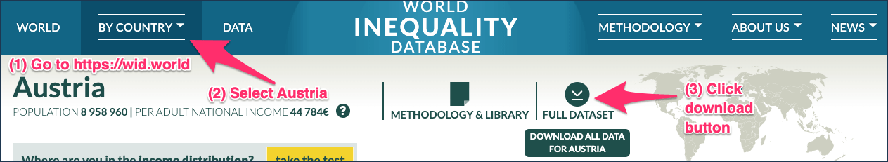
Click at the button “Full Dataset” to start download.
Download the compressed ZIP file to an appropriate place on your hard disk. The file name WID_fulldataset_AT_30-08-2024_15_02_39.zip has the structure “WID” + “_fulldataset_” + country code + “_” + day-month-year + “-” + hour-minute-second + “.zip”. Every part of date and time consists of two numbers. The time is UTC, i.e. one hour or two (in summer time) before Austrian local time.
Decompress the ZIP file with the appropriate tool on your computer. The result is a folder with the same name but without the extension “.zip”.
Delete the “.zip” file.
Graph 2.1: Download the Austrian dataset “By Country” via the interactive web page
R Code 2.1 : Download data for Austria
Code
# compute only once (manually)file_path="data/chap02/WID_fulldataset_AT_30-08-2024_15_02_39/WID_data_AT.csv"WID_data_AT<-readr::read_delim(file_path, delim =";", escape_double =FALSE, trim_ws =TRUE)pb_save_data_file("chap02", WID_data_AT, "WID_data_AT.rds")
Go straight (without selecting data) to the button “Download Full Dataset” and click it.
Download the compressed ZIP file to an appropriate place on your hard disk. The file name is wid_all_data.zip.
Decompress the ZIP file with the appropriate tool on your computer. The result is a folder with the same name but without the extension “.zip”.
Delete the “.zip” file.
Add the path of the huge wid_all_data folder (2.38 GB) to .gitignore because you don’t want to store all these files in your GitHub repo. Whenever you need a file to work on copy it programmatically in those areas that will be saved with Git.
Graph 2.2: Download the full WID dataset
2.3 Inspect downloaded folder
Graph 2.3: Screenshot of the ‘Files’ pane showing the content of the downloaded data folder
The data folder for the Austrian data has four files. The most important is the README.md file, because it explains very detailed the content of the other three files.
The data folder for the full WID data is in its structure not different. It contains one README.md and WID_countries.csv files with the same content as in the country downloaded version. The big difference is that there many WID_data_XX.csv and WID_metadata_XX.csv files. For each country code there is a file with the same structure as in the Austrian example meaning that WID_data_AT.csv has identical name and content in the “By Country” and the full version. Currently (2024-08-30) there are 338 “country” codes, include not only countries but smaller regions with (federal) states (like Alabama in the US and Bavaria in Germany) or larger region with geographical / political areas (like Europe and European Union).
2.4 Exploration of the README.md file
The README.md file contains information that is essential to understand the data structure. I will copy most of the content slightly changed for formatting reasons and add my own comments whenever I feel it is necessary.
2.4.1 Structure and Format of the CSV files
The CSV files use the semicolon “;” as a separator. Strings are quoted when required. The first row corresponds to variable names.
This is important information how to upload the .csv files. CSV stands for comma-separated values but in the WID case the separation character is a semi-colon. Instead of using the readr::read_csv() we have to use the more general readr::read_delim() function and specifying the delimiter as “;”.
2.4.1.1 Structure of WID_countries.csv file
The WID_countries.csv file contains five variables:
alpha2: the 2-letter country/region code. It mostly follows the ISO 3166-1 alpha-2 nomenclature, with some additions to account for former countries, regions and subregions. Regions within country XX are indicated as XX-YY, where YY is the region code. World regions are indicated as XX and XX-MER, the first one using purchasing power parities (PPP), (the default) and the second one using market exchange rates (MER). See the technical note “Prices and currency conversions in WID.world” for details.
titlename: the name of the country/region as it would appear in an English sentence (i.e. including the definite article, if any).
shortname: the name of the country/region as it would appear on its own in English (i.e. excluding the definite article).
region: broad world region to which the country belongs (similar to the first-level division of the United Nations geoscheme).
region2: detailed world region to which the country belongs (similar to the second-level division of the United Nations geoscheme).
The United Nation Geoscheme of the United Nations used by the WID is a tool widely utilized by organizations and governments, promotes a detailed worldview by fragmenting continents into more manageable portions. Although initially designed for statistical purposes by the United Nations Statistics Division, its application has extended beyond this original intent. But it is not uncontroversial.
For the WID the country questions is not the all important question because it (tries to) includes all self-governed territories that both have substantial economic resources of their own. So it contains Palestine, Kosovo, Taiwan and many more territories not recognized as an country.
2.4.1.2 Structure of the WID_data_XX.csv files
The WID_data_XX.csv files contain seven variables:
variable: WID variable code (see below for details).
percentile: WID percentile code (see below for details).
year: the year of the data point.
value: the value of the data point.
age: code indicating the age group to which the data point refers to.
pop: code indicating the population unit to which the data point refers to.
2.4.1.3 Structure of the WID_metadata_XX.csv
The WID_metadata_XX.csv contains seventeen variables:
country: the country/region code.
variable: the variable code to which the metadata refer.
age: the code of the age group to which the population refer.
pop: the code of the population unit to which the population refer.
countryname: the name of the country/region as it would appear in an English sentence.
shortname: the name of the country/region as it would appear on its own in English.
simpledes: decription of the variable in plain English.
technicaldes: description of the variable via accounting identities.
shorttype: short description of the variable type (average, aggregate, share, index, etc.) in plain English.
longtype: longer, more detailed description of the variable type in plain English.
shortpop: short description of the population unit (individuals, tax units, equal-split, etc.) in plain English.
longpop: longer, more detailed description of the population unit in plain English.
shortage: short description of the age group (adults, full population, etc.) in plain English.
longage: longer, more detailed description of the age group in plain English.
unit: unit of the variable (the 3-letter currency code for monetary amounts).
source: The source(s) used to compute the data.
method: Methological details describing how the data was constructed and/or caveats.
2.4.2 How to Interpret Variable Codes?
The meaning of each variable is described in the metadata files. The complete WID variable codes (i.e. sptinc992j) obey to the following logic:
the first letter indicates the variable type (i.e. “s” for share).
the next five letters indicate the income/wealth/other concept (i.e. ptinc for pre-tax national income).
the next three digits indicate the age group (i.e. 992 for adults).
the last letter indicate the population unit (i.e. j for equal-split).
2.4.3 How to Interpret Percentile Codes?
There are two types of percentiles on WID.world : (1) group percentiles and (2) generalized percentiles. The interpretation of income (or wealth) average, share or threshold series depends on which type of percentile is looked at.
2.4.3.1 Group Percentiles
Group percentiles are defined as follows:
p0p50 (bottom 50% of the population),
p50p90 (next 40%),
p90p100 (top 10%),
p99p100 (top 1%),
deciles:
p0p10 (bottom 10% of the population, i.e. first decile),
p10p20 (next 10%, i.e. second decile),
p20p30 (next 10%, i.e. third decile),
p30p40 (next 10%, i.e. fourth decile),
p40p50 (next 10%, i.e. fifth decile),
p50p60 (next 10%, i.e. sixth decile),
p60p70 (next 10%, i.e. seventh decile),
p70p80 (next 10%, i.e. eighth decile),
p80p90 (next 10%, i.e. ninth decile),
p90p100 (next 10%, i.e. tenth decile, already emntioned under top 10%)
p0p90 (bottom 90%),
p0p99 (bottom 99% of the population),
p99.9p100 (top 0.1%),
p99.99p100 (top 0.01%).
For each group percentiles, we provide the associated income or wealth shares, averages and thresholds.
group percentile shares correspond to the income (or wealth) share held by a given group percentile. For instance, the fiscal income share of group p0p50 is the share of total fiscal income captured by the bottom 50% group.
group percentile averages correspond to the income or wealth annual income (or wealth) average within a given group percentile group. For instance, the fiscal income average of group p0p50 is the average annual fiscal income of the bottom 50% group.
group percentile thresholds correspond to the minimum income (or wealth) level required to belong to a given group percentile. For instance, the fiscal income threshold of group p90p100 is the minimum annual fiscal income required to belong to the top 10% group.
When the data allows, the WID.world website makes it possible to produce shares, averages and thresholds for any group percentile (say, for instance, average income of p43p99.92). These are not stored in bulk data tables.
For certain countries, because of data limitations, we are not able to provide the list of group percentiles described above. We instead store specific group percentiles (these can be, depending on the countries p90p95, p95p100, p95p99, p99.5p100, p99.5p99.9, p99.75p100, p99.95p100, p99.95p99.99, p99.995p100, p99.9p99.95, p99.9p99.99 or p99p99.5).
2.4.3.2 Generalized Percentiles
Generalized percentiles (g-percentiles) are defined to as follows: p0, p1, p2, …, p99, p99.1, p99.2, …, p99.9, p99.91, p99.92, …, p99.99, p99.991, p99.992 ,…, p99.999. There are 127 g-percentiles in total.
For each g-percentiles, we provide shares, averages, top averages and thresholds.
g-percentiles shares correspond to the income (or wealth) share captured by the population group above a given g-percentile value. For example, the fiscal income share of g-percentile p90 corresponds to the fiscal income share held by the top 10% group; the fiscal income share of g-percentile p99.9 corresponds to the fiscal income share of the top 0.1% income group and so on. By construction, the fiscal income share of g-percentile p0 corresponds to the share held by 100% of the population and is equal to 100%. Formally, the g-percentile share at g-percentile pX corresponds to the share of the top (100-X)% group.
g-percentile averages correspond to the average income or wealth between two consecutive g-percentiles.
1% population group: Average income of g-percentile p0 corresponds to the average annual income of the bottom 1% group, p2 corresponds to the next 1% group and so on until p98 (the 1% population group below the top 1%).
Bottom 10% group of earners within the top 1% group of earners: Average income of g-percentile p99 corresponds to average annual of group percentile p99p99.1 (i.e. the bottom 10% group of earners within the top 1% group of earners), p99.1 corresponds to the next 0.1% group, p99.2 corresponds to the next 0.1% group and so on until p99.8.
Bottom 10% group of earners within the top 0.1% group of earners: Average income of p99.9 corresponds to the average annual income of group percentile p99.9p99.91 (i.e. the bottom 10% group of earners within the top 0.1% group of earners), p99.91 corresponds to the next 0.01% group, p99.92 corresponds to the next 0.01% group and so on until p99.98.
Bottom 10% group within the top 0.01% group of earners: Average income of p99.99, corresponds to the average annual income of group percentile p99.99p99.991 (i.e. the bottom 10% group within the top 0.01% group of earners), p99.991 corresponds to the next 0.001%, p99.992 corresponds to the next 0.001% group and so on until p99.999 (average income of the top 0.001% group).
For instance, average fiscal income of g-percentile p50 is equal to the average annual fiscal income of the p50p51 group percentile (i.e. the average annual income of the population group earning more than 50% of the population and less than the top 49% of the population). The average fiscal income of g-percentile p99 is equal to the average annual fiscal income within group percentile p99p99.1 (i.e. a group representing 0.1% of the total population earning more than 99% of the population but less than the top 0.9% of the population).
g-percentile top-averages correspond to the average income or wealth above a given g-percentile threshold. For instance the top average fiscal income at g-percentile p50 corresponds to the average annual fiscal income of individuals earning more than 50% of the population. The top average fiscal income at g-percentile p90 corresponds to the average annual fiscal income of the top 10% group.
g-percentile thresholds correspond to minimum income (or wealth) level required to belong to the population group above a given g-percentile value. For instance, the fiscal income threshold at g-percentile p90 corresponds to the minimum annual fiscal income required to belong to the top 10% group. Fiscal income threshold at g-percentile p99.9 corresponds to the minimum annual fiscal income required to belong to the top 0.1% group. Formally, the g-percentile threshold at g-percentile pX corresponds to the threshold of the top (100-X)% group.
Comparing with the letters used for the series types only “f” (female population) and “p” (proportion of women) are mssing in the Austrian dataset.
2.6 Trial to work with data
I am going to try different methods to work with the data from the WID. I will use as a prototypical example the Austrian income inequality during 1980-2022 of the pre-tax national income for the bottom 50%, middle 40%, top 10%, and top 1%.
2.6.1 Interactive website
2.6.1.1 Preparing the graph interactively
I have prepared the above mentioned task at the interactive WID website. The middle 40% is missing in the key indicators, so I had to use the menu “MORE INDICATORS”, Here is the screenshot of my result:
Graph 2.4: title
Sharing the results
Clicking at the top right arrow opens the option “Share” that offers several possibilities to disseminate the result.
Graph 2.5: title
2.6.1.2 iframe
The iframe option does not work. I do not know why this is the case. The standard reason for a “refused to connect” error occurs when the website being embedded has an X-Frame-Options policy set to restrict embedding in an iframe. But this shouldn’t be the case because the iframe code is offered freely at the WID interactive website.
Following the link the WID website will construct the graph and provide other information for further explorations (averages in absolute and threshold of the start amount of population group in currency units, and the beta coefficient), the full sharing set from the interactive construction website, the possibility to download the data and a detailed description of the variables (in plain English and more technical via account identities)
Note 2.1: Beta coefficient general in finance sectors and in WID particularly
The concept of beta coefficient, typically used in finance to measure market sensitivity, is not directly applicable to WID.world’s data. WID.world focuses on estimating and analyzing income and wealth inequality, not market returns or portfolio performance.
However, if we were to interpret the beta coefficient in a broader sense, considering the database’s focus on inequality, we could think of it as a measure of the sensitivity of income or wealth inequality to changes in macroeconomic variables, such as GDP growth, inflation, or interest rates.
In this context, the beta coefficient would represent the relationship between changes in these macroeconomic variables and the corresponding changes in income or wealth inequality. A high beta coefficient would indicate that income or wealth inequality is highly sensitive to changes in these macroeconomic variables, while a low beta coefficient would suggest a weaker relationship.
2.6.1.4 Image
Another option is to download a static graphic in JPG format from the WID website. It is a nice summary but has not as many options to refine, explore and get meta information as the URL in Section 2.6.1.3.
Graphic provided by the WID interactive website. (I have converted the JPG image to PNG format.)
2.6.1.5 Social media
Additionally you can post the result of your work on your Twitter or Facebook account.
2.6.2 Using the {wid} R package
Before I knew that the {wid} package will not be supported anymore (read the recent notice at the start of the README file on the GitHub repository by Thomas Blanchet1), I have used for my first trial the wid::download_wid() function. It worked fine and I hope that there will in the future another maintainer for this useful package.
R Code 2.4 : Download Austrian pre-tax income data using the {wid} package
Code
# download from WID only once (manually)sptincj992_wid_AT_50_40_10_1<-wid::download_wid( indicators ="sptinc", # Shares of pre-tax national income areas ="AT", # Austria perc =c("p0p50", # bottom 50%"p50p90", # middle 40%"p90p100", # top 10%"p99p100"# top 1%))pb_save_data_file("chap02", sptincj992_wid_AT_50_40_10_1, "sptincj992_wid_AT_50_40_10_1.rds")
(For this R code chunk is no output available)
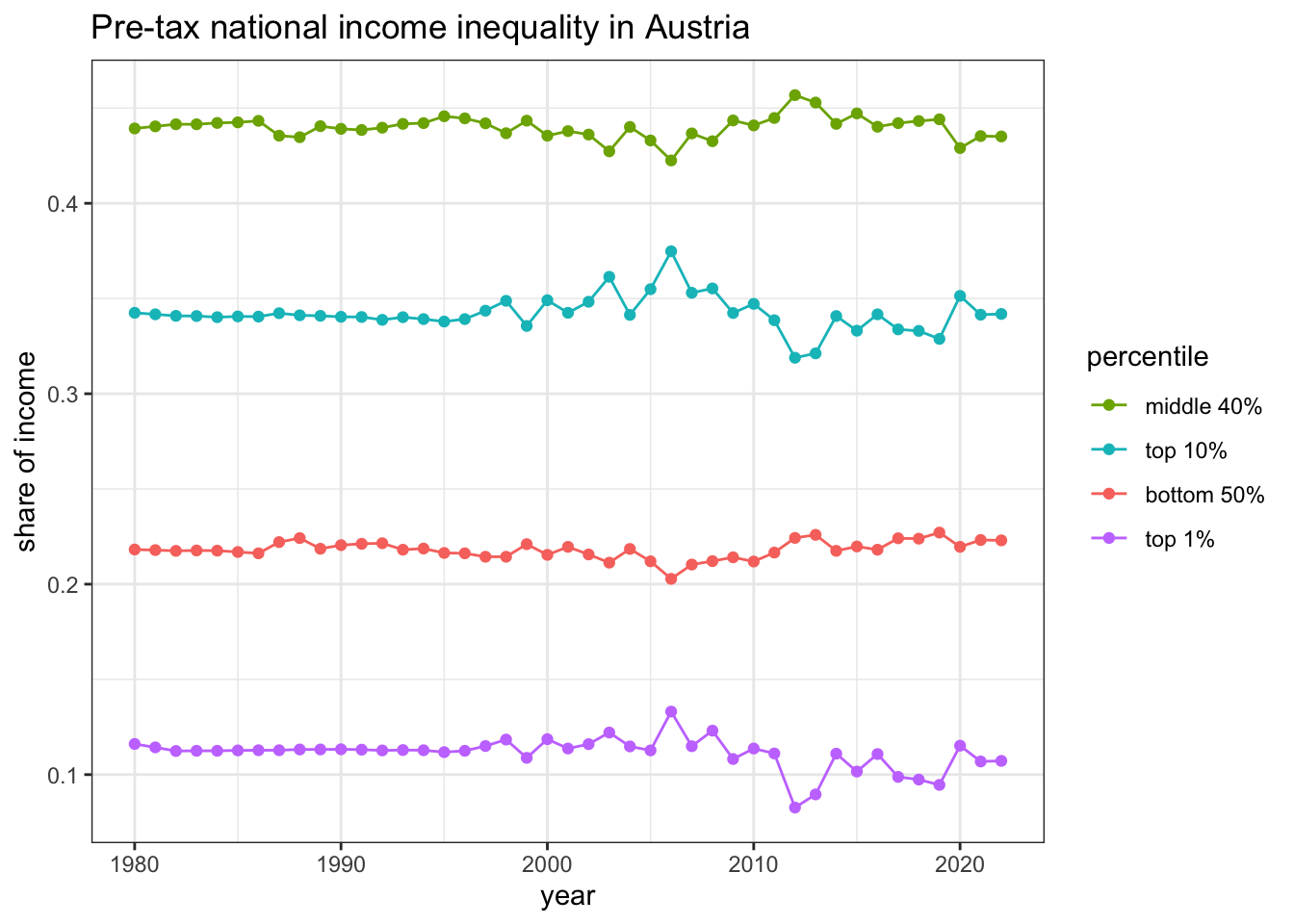
R Code 2.5 : Pre-tax national income for Austria (using {wid})
Listing / Output 2.1: Pre-tax national income for Austria (using {wid})
Code
sptincj992_wid_AT_50_40_10_1<-base::readRDS("data/chap02/sptincj992_wid_AT_50_40_10_1.rds")ggplot2::ggplot(sptincj992_wid_AT_50_40_10_1, ggplot2::aes(x =year, y =value, color =percentile))+ggplot2::geom_line()+ggplot2::geom_point()+ggplot2::ylab("share of income")+ggplot2::scale_color_discrete( breaks =c('p50p90', 'p90p100', 'p0p50', 'p99p100'), labels =c("p99p100"="top 1%","p0p50"="bottom 50%", "p90p100"="top 10%", "p50p90"="middle 40%"),)+ggplot2::ggtitle("Pre-tax national income inequality in Austria")
2.6.3 Using data form the original country file
Using the data directly from the original country file is the most general option with the highest flexibility. But to get a similar interactive graph one not has to use for the plot additionally to the {ggplot2} as shown in R Code 2.5 also the {plotly} package.
Taking this codes together results in the variable sptincj992.
I need the following percentiles:
bottom 50%: p0p50,
middle 40%: p50p90,
top 10% : p90p100,
top 1% : p99p100
R Code 2.6 : Preparing Austrian data for pre-tax national income (using country file)
Code
# compute only once (manually)WID_data_AT<-base::readRDS("data/chap02/WID_data_AT.rds")sptincj992_country_AT_50_40_10_1<-WID_data_AT|>dplyr::filter(variable=="sptincj992"&(percentile=="p0p50"|percentile=="p50p90"|percentile=="p90p100"|percentile=="p99p100"))|>dplyr::select(1:5)pb_save_data_file("chap02", sptincj992_country_AT_50_40_10_1, "sptincj992_country_AT_50_40_10_1.rds")
(For this R code chunk is no output available)
R Code 2.7 : Plot Austrian pre-tax national income (using country file)
Listing / Output 2.2: Plot Austrian pre-tax national income (using country file)
Code
sptincj992_country_AT_50_40_10_1<-base::readRDS("data/chap02/sptincj992_country_AT_50_40_10_1.rds")fig_sptincj992<-ggplot2::ggplot(sptincj992_country_AT_50_40_10_1, ggplot2::aes(x =year, y =value, color =percentile))+ggplot2::geom_line()+ggplot2::geom_point()+ggplot2::ylab("share of income")+ggplot2::scale_color_discrete( breaks =c('p50p90', 'p90p100', 'p0p50', 'p99p100'), labels =c("p99p100"="top 1%","p0p50"="bottom 50%", "p90p100"="top 10%", "p50p90"="middle 40%"),)+ggplot2::ggtitle("Pre-tax national income inequality in Austria")fig_sptincj992
Compare {wid} download with country data
We got the same results for our own computation from the original country file above with the calculation using the {wid} package Listing / Output 2.1. (Hover over the link to compare both graphs.)
There is no direct link to this section. The URL #first-letter-code` is not unique. It is used for the series type which comes before the population unit with the same URL.↩︎
Source Code
# Austrian Data {#sec-austrian-data}```{r}#| label: setup#| results: hold#| include: falsebase::source(file =paste0(here::here(), "/R/helper.R"))ggplot2::theme_set(ggplot2::theme_bw())```::: {#obj-chapter-template}::: my-objectives::: my-objectives-headerMy objective for this chapter:::::: my-objectives-containerIn this chapter, I will take a first take on the `r glossary("WID")`Austrian data set. I will import the dataset with two methods:1. "By Country" via the interactive web page.2. The full WID data set.Subsequently, I will explore the content of the data folder and describethe structure of the data.Finally, I will inspect the dataset and explore prototypically different methods to work with the data:- Using the interactive website (iframe, URL, image, social media)- Using the {**wid**} R package, which unfortunately recently is not supported anymore- Using the original country data files:::::::::## Import data by country::: my-procedure::: my-procedure-header::: {#prp-austrian-data-by-country}: Download the Austrian dataset "By Country" via the interactive webpage::::::::: my-procedure-container1. Go to the [WID homepage](https://wid.world/).2. Select "Austria" from the "By Country" menu.3. Click at the button "Full Dataset" to start download.4. Download the compressed `r glossary("ZIP")` file to an appropriate place on your hard disk. The file name`WID_fulldataset_AT_30-08-2024_15_02_39.zip` has the structure "WID" + "\_fulldataset\_" + `country code` + "\_" +`day-month-year` + "-" + `hour-minute-second` + ".zip". Every part of date and time consists of two numbers. The time is`r glossary("UTC")`, i.e. one hour or two (in summer time) before Austrian local time.5. Decompress the ZIP file with the appropriate tool on your computer. The result is a folder with the same name but without the extension ".zip".6. Delete the ".zip" file.::::::](img/02-download-austrian-data-by-country-skitch-min.png){#fig-02-austria-by-countryfig-alt="alt-text" fig-align="center" width="100%"}::: my-r-code::: my-r-code-header::: {#cnj-02-download-AT-data}: Download data for Austria::::::::: my-r-code-container```{r}#| label: download-AT-data#| eval: false# compute only once (manually)file_path ="data/chap02/WID_fulldataset_AT_30-08-2024_15_02_39/WID_data_AT.csv"WID_data_AT <- readr::read_delim(file_path, delim =";", escape_double =FALSE, trim_ws =TRUE)pb_save_data_file("chap02", WID_data_AT, "WID_data_AT.rds")```(*For this R code chunk is no output available*)::::::## Import the full WID dataset::: my-procedure::: my-procedure-header::: {#prp-complete-WID-data}: Download the full WID dataset::::::::: my-procedure-container1. Go to the [WID homepage](https://wid.world/).2. Select "Data" from the navigation bar.3. Go straight (without selecting data) to the button "Download Full Dataset" and click it.4. Download the compressed `r glossary("ZIP")` file to an appropriate place on your hard disk. The file name is `wid_all_data.zip`.5. Decompress the ZIP file with the appropriate tool on your computer. The result is a folder with the same name but without the extension ".zip".6. Delete the ".zip" file.7. Add the path of the huge `wid_all_data` folder (2.38 GB) to `.gitignore` because you don't want to store all these files in your GitHub repo. Whenever you need a file to work on copy it programmatically in those areas that will be saved with Git.::::::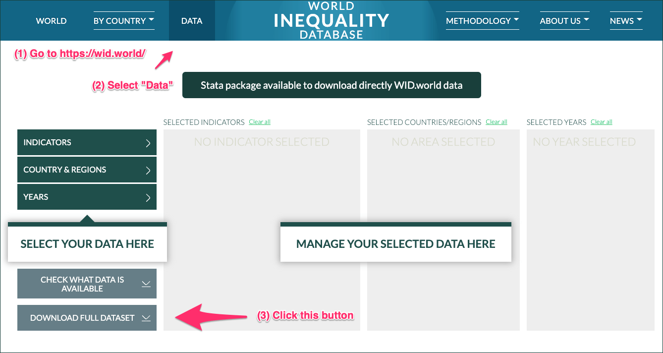{#fig-download-full-widfig-alt="alt-text" fig-align="center" width="100%"}## Inspect downloaded folder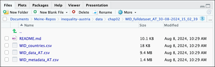{#fig-02-WID-AT-data-folderfig-alt="alt-text" fig-align="center" width="100%"}The data folder for the Austrian data has four files. The most importantis the `README.md` file, because it explains very detailed the contentof the other three files.The data folder for the full WID data is in its structure not different.It contains one `README.md` and `WID_countries.csv` files with the samecontent as in the country downloaded version. The big difference is thatthere many `WID_data_XX.csv` and `WID_metadata_XX.csv` files. For eachcountry code there is a file with the same structure as in the Austrianexample meaning that `WID_data_AT.csv` has identical name and content inthe "By Country" and the full version. Currently (2024-08-30) there are338 "country" codes, include not only countries but smaller regions with(federal) states (like Alabama in the US and Bavaria in Germany) orlarger region with geographical / political areas (like Europe andEuropean Union).## Exploration of the `README.md` fileThe `README.md` file contains information that is essential tounderstand the data structure. I will copy most of the content slightlychanged for formatting reasons and add my own comments whenever I feelit is necessary.### Structure and Format of the CSV files> The CSV files use the semicolon ";" as a separator. Strings are quoted> when required. The first row corresponds to variable names.This is important information how to upload the .csv files.`r glossary("CSV")` stands for comma-separated values but in the WIDcase the separation character is a semi-colon. Instead of using the`readr::read_csv()` we have to use the more general`readr::read_delim()` function and specifying the delimiter as ";".#### Structure of WID_countries.csv file {#sec-02-wid-countries}> The `WID_countries.csv` file contains five variables:>> - **alpha2**: the 2-letter country/region code. It mostly follows> the [ISO 3166-1 alpha-2> nomenclature](https://en.wikipedia.org/wiki/ISO_3166-1_alpha-2),> with some additions to account for former countries, regions and> subregions. Regions within country XX are indicated as XX-YY,> where YY is the region code. World regions are indicated as XX and> XX-MER, the first one using purchasing power parities> (`r glossary("PPP")`), (the default) and the second one using> market exchange rates (`r glossary("MER")`). See [the technical> note "Prices and currency conversions in> WID.world"](https://wid.world/document/convert-wid-world-series/)> for details.> - **titlename**: the name of the country/region as it would appear> in an English sentence (i.e. including the definite article, if> any).> - **shortname**: the name of the country/region as it would appear> on its own in English (i.e. excluding the definite article).> - **region**: broad world region to which the country belongs> (similar to the first-level division of the [United Nations> geoscheme](https://www.worldatlas.com/geography/the-geoscheme-of-the-united-nations.html)).> - **region2**: detailed world region to which the country belongs> (similar to the second-level division of the United Nations> geoscheme).The [United Nation Geoscheme of the UnitedNations](https://www.worldatlas.com/geography/the-geoscheme-of-the-united-nations.html)used by the WID is a tool widely utilized by organizations andgovernments, promotes a detailed worldview by fragmenting continentsinto more manageable portions. Although initially designed forstatistical purposes by the United Nations Statistics Division, itsapplication has extended beyond this original intent. But it is notuncontroversial.For example there is a recognition differences for Palestine and Kosovo.The UN recognizes [195 countries](https://www.worldatlas.com/countries):193 that belong to the United Nations (UN) plus the Holy See (Vatican)and the State of Palestine, which are non-member observer states. Seethe discussion in [How many countries are there in theworld](https://www.worldatlas.com/geography/how-many-countries-are-there-in-the-world.html)with a [list of countries according to the UNgeoscheme](https://www.worldatlas.com/geography/the-geoscheme-of-the-united-nations.html#h_27924556326881689241385858)and the [Official CountryList](https://www.worldatlas.com/geography/how-many-countries-are-there-in-the-world.html#h_8513270116691681224109796).For the WID the country questions is not the all important questionbecause it (tries to) includes all self-governed territories that bothhave substantial economic resources of their own. So it containsPalestine, Kosovo, Taiwan and many more territories not recognized as ancountry.#### Structure of the WID_data_XX.csv files> The WID_data_XX.csv files contain seven variables:>> - **country**: country/region code (see @sec-02-wid-countries).> - **variable**: WID variable code (see below for details).> - **percentile**: WID percentile code (see below for details).> - **year**: the year of the data point.> - **value**: the value of the data point.> - **age**: code indicating the age group to which the data point> refers to.> - **pop**: code indicating the population unit to which the data> point refers to.#### Structure of the WID_metadata_XX.csv> The WID_metadata_XX.csv contains seventeen variables:>> - **country**: the country/region code.> - **variable**: the variable code to which the metadata refer.> - **age**: the code of the age group to which the population refer.> - **pop**: the code of the population unit to which the population> refer.> - **countryname**: the name of the country/region as it would appear> in an English sentence.> - **shortname**: the name of the country/region as it would appear> on its own in English.> - **simpledes**: decription of the variable in plain English.> - **technicaldes**: description of the variable via accounting> identities.> - **shorttype**: short description of the variable type (average,> aggregate, share, index, etc.) in plain English.> - **longtype**: longer, more detailed description of the variable> type in plain English.> - **shortpop**: short description of the population unit> (individuals, tax units, equal-split, etc.) in plain English.> - **longpop**: longer, more detailed description of the population> unit in plain English.> - **shortage**: short description of the age group (adults, full> population, etc.) in plain English.> - **longage**: longer, more detailed description of the age group in> plain English.> - **unit**: unit of the variable (the 3-letter currency code for> monetary amounts).> - **source**: The source(s) used to compute the data.> - **method**: Methological details describing how the data was> constructed and/or caveats.### How to Interpret Variable Codes?> The meaning of each variable is described in the metadata files. The> complete WID variable codes (i.e. `sptinc992j`) obey to the following> logic:>> - **the first letter** indicates the variable type (i.e. "s" for> share).> - **the next five letters** indicate the income/wealth/other concept> (i.e. `ptinc` for pre-tax national income).> - **the next three digits** indicate the age group (i.e. `992` for> adults).> - **the last letter** indicate the population unit (i.e. `j` for> equal-split).### How to Interpret Percentile Codes?There are two types of percentiles on WID.world : (1) group percentilesand (2) generalized percentiles. The interpretation of income (orwealth) average, share or threshold series depends on which type ofpercentile is looked at.#### Group Percentiles> Group percentiles are defined as follows:>> - p0p50 (bottom 50% of the population),> - p50p90 (next 40%),> - p90p100 (top 10%),> - p99p100 (top 1%),> - deciles:> - p0p10 (bottom 10% of the population, i.e. first decile),> - p10p20 (next 10%, i.e. second decile),> - p20p30 (next 10%, i.e. third decile),> - p30p40 (next 10%, i.e. fourth decile),> - p40p50 (next 10%, i.e. fifth decile),> - p50p60 (next 10%, i.e. sixth decile),> - p60p70 (next 10%, i.e. seventh decile),> - p70p80 (next 10%, i.e. eighth decile),> - p80p90 (next 10%, i.e. ninth decile),> - p90p100 (next 10%, i.e. tenth decile, already emntioned under> top 10%)> - p0p90 (bottom 90%),> - p0p99 (bottom 99% of the population),> - p99.9p100 (top 0.1%),> - p99.99p100 (top 0.01%).>> For each group percentiles, we provide the associated income or wealth> shares, averages and thresholds.>> - **group percentile shares** correspond to the income (or wealth)> share held by a given group percentile. For instance, the> fiscal income share of group p0p50 is the share of total fiscal> income captured by the bottom 50% group.> - **group percentile averages** correspond to the income or wealth> annual income (or wealth) average within a given group percentile> group. For instance, the fiscal income average of group p0p50 is> the average annual fiscal income of the bottom 50% group.> - **group percentile thresholds** correspond to the minimum income> (or wealth) level required to belong to a given group> percentile. For instance, the fiscal income threshold of group> p90p100 is the minimum annual fiscal income required to belong to> the top 10% group.>> When the data allows, the WID.world website makes it possible> to produce shares, averages and thresholds for any group percentile> (say, for instance, average income of p43p99.92). These are not stored> in bulk data tables.>> For certain countries, because of data limitations, we are not able to> provide the list of group percentiles described above. We instead> store specific group percentiles (these can be, depending on the> countries p90p95, p95p100, p95p99, p99.5p100, p99.5p99.9, p99.75p100,> p99.95p100, p99.95p99.99, p99.995p100, p99.9p99.95, p99.9p99.99 or> p99p99.5).#### Generalized Percentiles> **Generalized percentiles (g-percentiles)** are defined to as follows:> p0, p1, p2, ..., p99, p99.1, p99.2, ..., p99.9, p99.91, p99.92, ...,> p99.99, p99.991, p99.992 ,..., p99.999. There are 127 g-percentiles in> total.>> For each g-percentiles, we provide shares, averages, top averages and> thresholds.>> - **g-percentiles shares** correspond to the income (or wealth)> share captured by the population group above a given g-percentile> value. For example, the fiscal income share of g-percentile p90> corresponds to the fiscal income share held by the top 10% group;> the fiscal income share of g-percentile p99.9 corresponds to the> fiscal income share of the top 0.1% income group and so on. By> construction, the fiscal income share of g-percentile p0> corresponds to the share held by 100% of the population and is> equal to 100%. Formally, the g-percentile share at g-percentile pX> corresponds to the share of the top (100-X)% group.> - **g-percentile averages** correspond to the average income or> wealth between two consecutive g-percentiles.> - **1% population group**: Average income of g-percentile p0> corresponds to the average annual income of the bottom 1%> group, p2 corresponds to the next 1% group and so on until p98> (the 1% population group below the top 1%).> - **Bottom 10% group of earners within the top 1% group of> earners**: Average income of g-percentile p99 corresponds to> average annual of group percentile p99p99.1 (i.e. the bottom> 10% group of earners within the top 1% group of earners),> p99.1 corresponds to the next 0.1% group, p99.2 corresponds to> the next 0.1% group and so on until p99.8.> - **Bottom 10% group of earners within the top 0.1% group of> earners**: Average income of p99.9 corresponds to the average> annual income of group percentile p99.9p99.91 (i.e. the bottom> 10% group of earners within the top 0.1% group of earners),> p99.91 corresponds to the next 0.01% group, p99.92 corresponds> to the next 0.01% group and so on until p99.98.> - **Bottom 10% group within the top 0.01% group of earners**:> Average income of p99.99, corresponds to the average annual> income of group percentile p99.99p99.991 (i.e. the bottom 10%> group within the top 0.01% group of earners), p99.991> corresponds to the next 0.001%, p99.992 corresponds to the> next 0.001% group and so on until p99.999 (average income of> the top 0.001% group).>> For instance, average fiscal income of g-percentile p50 is equal to> the average annual fiscal income of the p50p51 group percentile (i.e.> the average annual income of the population group earning more than> 50% of the population and less than the top 49% of the population).> The average fiscal income of g-percentile p99 is equal to the average> annual fiscal income within group percentile p99p99.1 (i.e. a group> representing 0.1% of the total population earning more than 99% of the> population but less than the top 0.9% of the population).>> - **g-percentile top-averages** correspond to the average income or> wealth above a given g-percentile threshold. For instance the top> average fiscal income at g-percentile p50 corresponds to the> average annual fiscal income of individuals earning more than 50%> of the population. The top average fiscal income at g-percentile> p90 corresponds to the average annual fiscal income of the top 10%> group.> - **g-percentile thresholds** correspond to minimum income (or> wealth) level required to belong to the population group above a> given g-percentile value. For instance, the fiscal income> threshold at g-percentile p90 corresponds to the minimum annual> fiscal income required to belong to the top 10% group. Fiscal> income threshold at g-percentile p99.9 corresponds to the minimum> annual fiscal income required to belong to the top 0.1% group.> Formally, the g-percentile threshold at g-percentile pX> corresponds to the threshold of the top (100-X)% group.## Inspect AT data### Summary look at the data::: my-r-code::: my-r-code-header::: {#cnj-02-skim-AT-data}: Look at the AT dataset::::::::: my-r-code-container```{r}#| label: skim-AT-dataWID_AT <- base::readRDS("data/chap02/WID_data_AT.rds")skimr::skim(WID_AT)```::::::### Explore types of series:::::{.my-r-code}:::{.my-r-code-header}:::::: {#cnj-02-count-series-types}: Distribution of series types for Austrian Data:::::::::::::{.my-r-code-container}```{r}#| label: count-series-typesWID_AT |> dplyr::mutate(series =substr(variable, 1, 1)) |> dplyr::count(series) |> DT::datatable()```´:::::::::Comparing with the letters used for the series types only "f" (female population) and "p" (proportion of women) are mssing in the Austrian dataset.## Trial to work with dataI am going to try different methods to work with the data from the WID.I will use as a prototypical example the Austrian income inequalityduring 1980-2022 of the pre-tax national income for the bottom 50%,middle 40%, top 10%, and top 1%.### Interactive website#### Preparing the graph interactivelyI have prepared the above mentioned task at the interactive WID website.The middle 40% is missing in the key indicators, so I had to use themenu "MORE INDICATORS", Here is the screenshot of my result: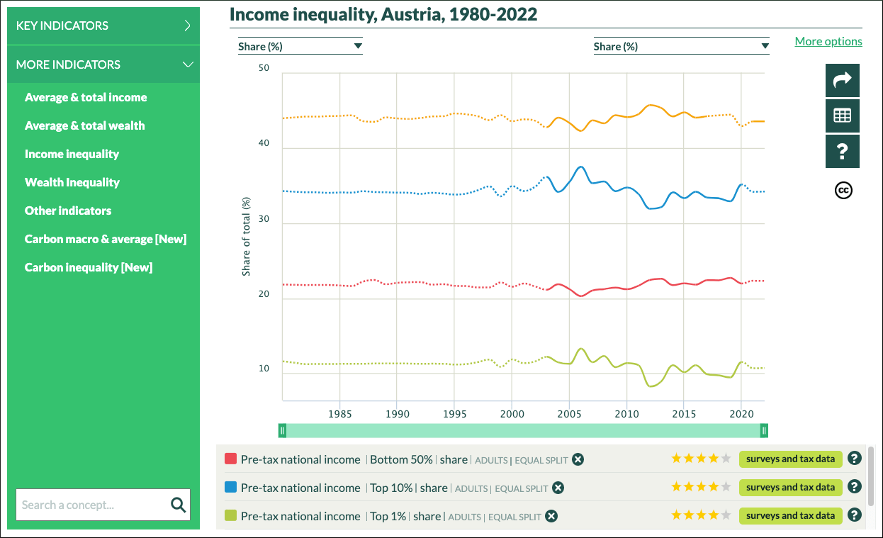{#fig-02-screenshot-income_WID_AT_50_40_10_1fig-alt="alt-text" fig-align="center" width="100%"}Sharing the resultsClicking at the top right arrow opens the option "Share" that offersseveral possibilities to disseminate the result.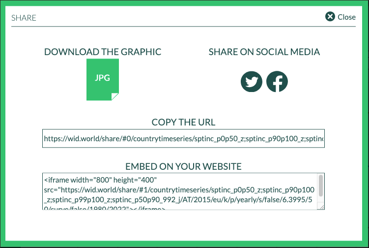{#fig-14-04fig-alt="alt-text" fig-align="center" width="100%"}#### iframe<iframe width="800" height="400" src="https://wid.world/share/#1/countrytimeseries/sptinc_p0p50_z;sptinc_p90p100_z;sptinc_p99p100_z;sptinc_p50p90_992_j/AT/2015/eu/k/p/yearly/s/false/6.3995/50/curve/false/1980/2022"></iframe>The `r glossary("iframe")` option does not work. I do not know why thisis the case. The standard reason for a “refused to connect” error occurswhen the website being embedded has an X-Frame-Options policy set torestrict embedding in an iframe. But this shouldn't be the case becausethe iframe code is offered freely at the WID interactive website.#### URL {#sec-02-url-provided-by-WID}[URL provided by interactive WIDwebsite](https://wid.world/share/#0/countrytimeseries/sptinc_p0p50_z;sptinc_p90p100_z;sptinc_p99p100_z;sptinc_p50p90_992_j/AT/2015/eu/k/p/yearly/s/false/6.3995/50/curve/false/1980/2022){fig-alt="alt-text"fig-align="center" width="100%"}Following the link the WID website will construct the graph and provideother information for further explorations (averages in absolute andthreshold of the start amount of population group in currency units, andthe `r glossary("beta coefficient")`), the full sharing set from theinteractive construction website, the possibility to download the dataand a detailed description of the variables (in plain English and moretechnical via account identities)::: {#nte-beta-coefficient .callout-note}####### Beta coefficient general in finance sectors and in WID particularlyThe concept of beta coefficient, typically used in finance to measuremarket sensitivity, is not directly applicable to WID.world’s data.WID.world focuses on estimating and analyzing income and wealthinequality, not market returns or portfolio performance.However, if we were to interpret the beta coefficient in a broadersense, considering the database’s focus on inequality, we could think ofit as a measure of the sensitivity of income or wealth inequality tochanges in macroeconomic variables, such as GDP growth, inflation, orinterest rates.In this context, the beta coefficient would represent the relationshipbetween changes in these macroeconomic variables and the correspondingchanges in income or wealth inequality. A high beta coefficient wouldindicate that income or wealth inequality is highly sensitive to changesin these macroeconomic variables, while a low beta coefficient wouldsuggest a weaker relationship.:::#### ImageAnother option is to download a static graphic in `r glossary("JPG")`format from the WID website. It is a nice summary but has not as manyoptions to refine, explore and get meta information as the URL in@sec-02-url-provided-by-WID.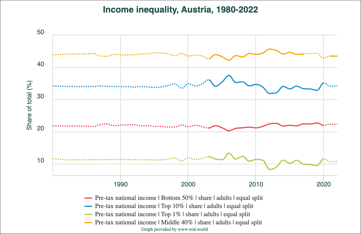{fig-alt="alt-text"fig-align="center" width="100%"}#### Social mediaAdditionally you can post the result of your work on your Twitter orFacebook account.### Using the {wid} R packageBefore I knew that the {**wid**} package will not be supported anymore(read the recent notice at the start of the [README file on the GitHubrepository](https://github.com/thomasblanchet/wid-r-tool) by ThomasBlanchet[^02-austrian-data-1]), I have used for my first trial the`wid::download_wid()` function. It worked fine and I hope that therewill in the future another maintainer for this useful package.[^02-austrian-data-1]: Author and Maintainer [Thomas Blanchet has changed jobs](https://github.com/thomasblanchet) and is not affiliated anymore with the `r glossary("WIL")`.::: my-r-code::: my-r-code-header::: {#cnj-02-download-sptincj992-wid-AT-50-40-10-1}: Download Austrian pre-tax income data using the {**wid**} package::::::::: my-r-code-container```{r}#| label: download-sptincj992-wid-AT-50-40-10-1#| eval: false# download from WID only once (manually)sptincj992_wid_AT_50_40_10_1 <- wid::download_wid(indicators ="sptinc", # Shares of pre-tax national incomeareas ="AT", # Austriaperc =c("p0p50", # bottom 50%"p50p90", # middle 40%"p90p100", # top 10%"p99p100"# top 1% ))pb_save_data_file("chap02", sptincj992_wid_AT_50_40_10_1, "sptincj992_wid_AT_50_40_10_1.rds")```(*For this R code chunk is no output available*)::::::::: my-r-code::: my-r-code-header::: {#cnj-02-plot-sptincj992-wid-AT-50-40-10-1}: Pre-tax national income for Austria (using {wid})::::::::: my-r-code-container::: {#lst-02-plot-sptincj992_wid_AT_50_40_10_1}```{r}#| label: plot-sptincj992-wid-AT-50-40-10-1sptincj992_wid_AT_50_40_10_1 <- base::readRDS("data/chap02/sptincj992_wid_AT_50_40_10_1.rds")ggplot2::ggplot(sptincj992_wid_AT_50_40_10_1, ggplot2::aes(x = year, y = value, color = percentile)) + ggplot2::geom_line() + ggplot2::geom_point() + ggplot2::ylab("share of income") + ggplot2::scale_color_discrete(breaks =c('p50p90', 'p90p100', 'p0p50', 'p99p100' ),labels =c("p99p100"="top 1%","p0p50"="bottom 50%", "p90p100"="top 10%", "p50p90"="middle 40%" ), ) + ggplot2::ggtitle("Pre-tax national income inequality in Austria")```Pre-tax national income for Austria (using {wid}):::::::::### Using data form the original country fileUsing the data directly from the original country file is the mostgeneral option with the highest flexibility. But to get a similarinteractive graph one not has to use for the plot additionally to the{**ggplot2**} as shown in @cnj-02-plot-sptincj992-wid-AT-50-40-10-1 alsothe {**plotly**} package.I need the following variable:- The [series type](https://wid.world/codes-dictionary/#one-letter-code) is "share" = `s`- The [pre-tax national income](https://wid.world/codes-dictionary/#pretax-income) =`ptinc`.- The population unit[^02-austrian-data-2] is "equal-split adults" = `j`.- The [adult population](https://wid.world/codes-dictionary/#three-digit-code) =`992`.[^02-austrian-data-2]: There is no direct link to this section. The URL`#first-letter-code`\` is not unique. It is used for the series type which comes before the population unit with the same URL.Taking this codes together results in the variable `sptincj992`.I need the following percentiles:- bottom 50%: `p0p50`,- middle 40%: `p50p90`,\- top 10% : `p90p100`,- top 1% : `p99p100`::: my-r-code::: my-r-code-header::: {#cnj-02-sptincj992_country_AT_50_40_10_1}: Preparing Austrian data for pre-tax national income (using country file)::::::::: my-r-code-container```{r}#| label: sptincj992_country_AT_50_40_10_1#| eval: false# compute only once (manually)WID_data_AT <- base::readRDS("data/chap02/WID_data_AT.rds")sptincj992_country_AT_50_40_10_1 <- WID_data_AT |> dplyr::filter( variable =="sptincj992"& ( percentile =="p0p50"| percentile =="p50p90"| percentile =="p90p100"| percentile =="p99p100") ) |> dplyr::select(1:5)pb_save_data_file("chap02", sptincj992_country_AT_50_40_10_1, "sptincj992_country_AT_50_40_10_1.rds")```(*For this R code chunk is no output available*):::::::::::{.my-r-code}:::{.my-r-code-header}:::::: {#cnj-02-plot-sptincj992_country_AT_50_40_10_1}: Plot Austrian pre-tax national income (using country file):::::::::::::{.my-r-code-container}::: {#lst-02-plot-sptincj992_country_AT_50_40_10_1}```{r}#| label: plot-sptincj992_country_AT_50_40_10_1sptincj992_country_AT_50_40_10_1 <- base::readRDS("data/chap02/sptincj992_country_AT_50_40_10_1.rds")fig_sptincj992 <- ggplot2::ggplot(sptincj992_country_AT_50_40_10_1, ggplot2::aes(x = year, y = value, color = percentile)) + ggplot2::geom_line() + ggplot2::geom_point() + ggplot2::ylab("share of income") + ggplot2::scale_color_discrete(breaks =c('p50p90', 'p90p100', 'p0p50', 'p99p100' ),labels =c("p99p100"="top 1%","p0p50"="bottom 50%", "p90p100"="top 10%", "p50p90"="middle 40%" ), ) + ggplot2::ggtitle("Pre-tax national income inequality in Austria")fig_sptincj992```Plot Austrian pre-tax national income (using country file)::::::::::::::: {.callout-tip}####### Compare {wid} download with country dataWe got the same results for our own computation from the original country file above with the calculation using the {**wid**} package @lst-02-plot-sptincj992_wid_AT_50_40_10_1. (Hover over the link to compare both graphs.)::::::::{.my-r-code}:::{.my-r-code-header}:::::: {#cnj-ID-text}: Numbered R Code Title:::::::::::::{.my-r-code-container}```{r}#| label: code-chunk-nameplotly::ggplotly(fig_sptincj992)```::::::::::::::{.my-resource}:::{.my-resource-header}:::::: {#lem-02-plotly-resources}: Plotly Resources for R:::::::::::::{.my-resource-container}- **Website**: Sievert, C. (2019). Interactive web-based data visualization with R, plotly, and shiny. [https://plotly-r.com/](https://plotly-r.com/)- **Book**: Sievert, C. (2020). Interactive Web-Based Data Visualization with R, plotly, and shiny. Chapman and Hall/CRC. [DOI](https://doi.org/10.1201/9780429447273).:::::::::


2.6.1.5 Social media
Additionally you can post the result of your work on your Twitter or Facebook account.