Mapping data & advanced visualization

You will learn how to:

• Work with spatial data
• Create interactive maps in Shiny using Leaflet
• Use Shiny events and proxies

1 Interactive maps

• Mapping is a type of data visualization based on spatial data
• Classic cartography relies on generalization and interpretation
• Interactive cartography removes many limitations such as generalization and map boundaries

Generalization in OpenStreetMap at different scales

1.1 Current app state

• Quick recap:
  • In section 3, we added an introduction tab that contains background info on the app
  • In section 4, we added a table tab using the DT package
  • In section 5, we added a modelling tab using all sorts of visualizations

Full code for the current app state

library(shiny)
library(htmltools)
library(bs4Dash)
library(fresh)
library(waiter)
library(shinyWidgets)
library(Guerry)
library(sf)
library(tidyr)
library(dplyr)
library(RColorBrewer)
library(viridis)
library(leaflet)
library(plotly)
library(ggplot2)
library(GGally)
library(datawizard)
library(parameters)
library(performance)
library(modelsummary)

# 1 Data preparation ----

## Load & clean data ----
variable_names <- list(
  Crime_pers = "Crime against persons",  
  Crime_prop =  "Crime against property",  
  Literacy = "Literacy",  
  Donations = "Donations to the poor",  
  Infants = "Illegitimate births",  
  Suicides = "Suicides",  
  Wealth = "Tax / capita",  
  Commerce = "Commerce & Industry",  
  Clergy = "Clergy",  
  Crime_parents = "Crime against parents",  
  Infanticide = "Infanticides",  
  Donation_clergy = "Donations to the clergy",  
  Lottery = "Wager on Royal Lottery",  
  Desertion = "Military desertion",  
  Instruction = "Instruction",  
  Prostitutes = "Prostitutes",  
  Distance = "Distance to paris",  
  Area = "Area",  
  Pop1831 = "Population"
)

data_guerry <- Guerry::gfrance85 %>%
  st_as_sf() %>%
  as_tibble() %>%
  st_as_sf(crs = 27572) %>%
  mutate(Region = case_match(
    Region,
    "C" ~ "Central",
    "E" ~ "East",
    "N" ~ "North",
    "S" ~ "South",
    "W" ~ "West"
  )) %>%
  select(-c("COUNT", "dept", "AVE_ID_GEO", "CODE_DEPT")) %>%
  select(Region:Department, all_of(names(variable_names)))



## Prep data (Tab: Tabulate data) ----
data_guerry_tabulate <- data_guerry %>% 
  st_drop_geometry() %>% 
  mutate(across(.cols = all_of(names(variable_names)), round, 2))


## Prep data (Tab: Map data) ----
data_guerry_region <- data_guerry %>%
  group_by(Region) %>%
  summarise(across(
    .cols = all_of(names(variable_names)),
    function(x) {
      if (cur_column() %in% c("Area", "Pop1831")) {
        sum(x)
      } else {
        mean(x)
      }
    }
  ))

## Prepare palettes ----
## Used for mapping
pals <- list(
  Sequential = RColorBrewer::brewer.pal.info %>%
    filter(category %in% "seq") %>%
    row.names(),
  Viridis = c("Magma", "Inferno", "Plasma", "Viridis",
              "Cividis", "Rocket", "Mako", "Turbo")
)

## Prepare modebar clean-up ----
## Used for modelling
plotly_buttons <- c(
  "sendDataToCloud", "zoom2d", "select2d", "lasso2d", "autoScale2d",
  "hoverClosestCartesian", "hoverCompareCartesian", "resetScale2d"
)




# 3 UI ----

ui <- dashboardPage(
  title = "The Guerry Dashboard",
  ## 3.1 Header ----
  header = dashboardHeader(
    title = tagList(
      img(src = "../workshop-logo.png", width = 35, height = 35),
      span("The Guerry Dashboard", class = "brand-text")
    )
  ),
  ## 3.2 Sidebar ----
  sidebar = dashboardSidebar(
    id = "sidebar",
    sidebarMenu(
      id = "sidebarMenu",
      menuItem(tabName = "tab_intro", text = "Introduction", icon = icon("home")),
      menuItem(tabName = "tab_tabulate", text = "Tabulate data", icon = icon("table")),
      menuItem(tabName = "tab_model", text = "Model data", icon = icon("chart-line")),
      menuItem(tabName = "tab_map", text = "Map data", icon = icon("map")),
      flat = TRUE
    ),
    minified = TRUE,
    collapsed = TRUE,
    fixed = FALSE,
    skin = "light"
  ),
  ## 3.3 Body ----
  body = dashboardBody(
    tabItems(
      ### 3.1.1 Tab: Introduction ----
      tabItem(
        tabName = "tab_intro",
        jumbotron(
          title = "The Guerry Dashboard",
          lead = "A Shiny app to explore the classic Guerry dataset.",
          status = "info",
          btnName = NULL
        ),
        fluidRow(
          column(width = 1),
          column(
            width = 6,
            box(
              title = "About",
              status = "primary",
              width = 12,
              blockQuote(HTML("André-Michel Guerry was a French lawyer and
                          amateur statistician. Together with Adolphe
                          Quetelet he may be regarded as the founder of
                          moral statistics which led to the development
                          of criminology, sociology and ultimately,
                          modern social science. <br>— Wikipedia: <a href='https://en.wikipedia.org/wiki/Andr%C3%A9-Michel_Guerry'>André-Michel Guerry</a>"),
                         color = "primary"),
              p(HTML("Andre-Michel Guerry (1833) was the first to 
              systematically collect and analyze social data 
               on such things as crime, literacy and suicide 
               with the view to determining social laws and the 
               relations among these variables. The Guerry data 
               frame comprises a collection of 'moral variables' 
               (cf. <i><a href='https://en.wikipedia.org/wiki/Moral_statistics'>moral statistics</a></i>) 
               on the 86 departments of France around 1830. 
               A few additional variables have been added 
               from other sources. In total the data frame has 
               86 observations (the departments of France) on 23 variables <i>(Source: <code>?Guerry</code>)</i>. 
               In this app, we aim to explore Guerry’s data
                using spatial exploration and regression modelling.")),
              hr(),
              accordion(
                id = "accord",
                accordionItem(
                  title = "References",
                  status = "primary",
                  solidHeader = FALSE,
                  "The following sources are referenced in this app:",
                  tags$ul(
                    class = "list-style: none",
                    style = "margin-left: -30px;",
                    p("Angeville, A. (1836). Essai sur la Statistique de la Population française Paris: F. Doufour."),
                    p("Guerry, A.-M. (1833). Essai sur la statistique morale de la France Paris: Crochard. English translation: Hugh P. Whitt and Victor W. Reinking, Lewiston, N.Y. : Edwin Mellen Press, 2002."),
                    p("Parent-Duchatelet, A. (1836). De la prostitution dans la ville de Paris, 3rd ed, 1857, p. 32, 36"),
                    p("Palsky, G. (2008). Connections and exchanges in European thematic cartography. The case of 19th century choropleth maps. Belgeo 3-4, 413-426.")
                  )
                ),
                accordionItem(
                  title = "Details",
                  status = "primary",
                  solidHeader = FALSE,
                  p("This app was created as part of a Shiny workshop held in July 2023"),
                  p("Last update: June 2023"),
                  p("Further information about the data can be found",
                    a("here.", href = "https://www.datavis.ca/gallery/guerry/guerrydat.html"))
                )
              )
            )
          ),
          column(
            width = 4,
            box(
              title = "André Michel Guerry",
              status = "primary",
              width = 12,
              tags$img(src = "../guerry.jpg", width = "100%"),
              p("Source: Palsky (2008)")
            )
          )
        )
      ),
      ### 3.3.2 Tab: Tabulate data ----
      tabItem(
        tabName = "tab_tabulate",
        fluidRow(
          #### Inputs(s) ----
          pickerInput(
            "tab_tabulate_select",
            label = "Filter variables",
            choices = setNames(names(variable_names), variable_names),
            options = pickerOptions(
              actionsBox = TRUE,
              windowPadding = c(30, 0, 0, 0),
              liveSearch = TRUE,
              selectedTextFormat = "count",
              countSelectedText = "{0} variables selected",
              noneSelectedText = "No filters applied"
            ),
            inline = TRUE,
            multiple = TRUE
          )
        ),
        hr(),
        #### Output(s) (Data table) ----
        DT::dataTableOutput("tab_tabulate_table")
      ),
      ### 3.3.3 Tab: Model data ----
      tabItem(
        tabName = "tab_model",
        fluidRow(
          column(
            width = 6,
            #### Inputs(s) ----
            box(
              width = 12,
              title = "Select variables",
              status = "primary",
              shinyWidgets::pickerInput(
                "model_x",
                label = "Select a dependent variable",
                choices = setNames(names(variable_names), variable_names),
                options = shinyWidgets::pickerOptions(liveSearch = TRUE),
                selected = "Literacy"
              ),
              shinyWidgets::pickerInput(
                "model_y",
                label = "Select independent variables",
                choices = setNames(names(variable_names), variable_names),
                options = shinyWidgets::pickerOptions(
                  actionsBox = TRUE,
                  liveSearch = TRUE,
                  selectedTextFormat = "count",
                  countSelectedText = "{0} variables selected",
                  noneSelectedText = "No variables selected"
                ),
                multiple = TRUE,
                selected = "Commerce"
              ),
              shinyWidgets::prettyCheckbox(
                "model_std",
                label = "Standardize variables?",
                value = TRUE,
                status = "primary",
                shape = "curve"
              ),
              hr(),
              actionButton(
                "refresh",
                label = "Apply changes",
                icon = icon("refresh"),
                flat = TRUE
              )
            ),
            #### Outputs(s) ----
            tabBox(
              status = "primary",
              type = "tabs",
              title = "Model analysis",
              side = "right",
              width = 12,
              ##### Tabpanel: Coefficient plot ----
              tabPanel(
                title = "Plot: Coefficients",
                plotly::plotlyOutput("coefficientplot")
              ),
              ##### Tabpanel: Scatterplot ----
              tabPanel(
                title = "Plot: Scatterplot",
                plotly::plotlyOutput("scatterplot")
              ),
              ##### Tabpanel: Table: Regression ----
              tabPanel(
                title = "Table: Model",
                htmlOutput("tableregression")
              )
            )
          ),
          column(
            width = 6,
            ##### Box: Pair diagramm ----
            box(
              width = 12,
              title = "Pair diagram",
              status = "primary",
              plotly::plotlyOutput("pairplot")
            ),
            ##### TabBox: Model diagnostics ----
            tabBox(
              status = "primary",
              type = "tabs",
              title = "Model diagnostics",
              width = 12,
              side = "right",
              tabPanel(
                title = "Normality",
                plotly::plotlyOutput("normality")
              ),
              tabPanel(
                title = "Outliers",
                plotly::plotlyOutput("outliers")
              ),
              tabPanel(
                title = "Heteroskedasticity",
                plotly::plotlyOutput("heteroskedasticity")
              )
            )
          )
        )
      ),
      ### 3.3.4 Tab: Map data ----
      tabItem(
        tabName = "tab_map", # must correspond to related menuItem name
        fluidRow(
          column(
            #### Output(s) ----
            width = 8,
            box(
              id = "tab_map_box",
              status = "primary",
              headerBorder = FALSE,
              collapsible = FALSE,
              width = 12,
              leaflet::leafletOutput("tab_map_map", height = "800px", width = "100%")
            ) # end box
          ) # end column
        ) # end fluidRow
      ) # end tabItem
    ) # end tabItems
  ),
  
  ## 3.4 Footer (bottom)----
  footer = dashboardFooter(
    left = span(
      "This dashboard was created by Jonas Lieth and Paul Bauer. Find the source code",
      a("here.", href = "https://github.com/paulcbauer/shiny_workshop/tree/main/shinyapps/guerry"),
      "It is based on data from the",
      a("Guerry R package.", href = "https://cran.r-project.org/web/packages/Guerry/index.html")
    )
  ),
  ## 3.5 Controlbar (top)----
  controlbar = dashboardControlbar(
    div(class = "p-3", skinSelector()),
    skin = "light"
  )  
)



# 4 Server ----

server <- function(input, output, session) {
  
  ## 4.1 Tabulate data ----
  ### Variable selection ----
  tab <- reactive({
    var <- input$tab_tabulate_select
    data_table <- data_guerry_tabulate
    
    if (!is.null(var)) {
      data_table <- data_table[, var]
    }
    
    data_table
  })
  
  
  ### Create table----
  dt <- reactive({
    tab <- tab()
    ridx <- ifelse("Department" %in% names(tab), 3, 1)
    DT::datatable(
      tab,
      class = "hover",
      extensions = c("Buttons"),
      selection = "none",
      filter = list(position = "top", clear = FALSE),
      style = "bootstrap4",
      rownames = FALSE,
      options = list(
        dom = "Brtip",
        deferRender = TRUE,
        scroller = TRUE,
        buttons = list(
          list(extend = "copy", text = "Copy to clipboard"),
          list(extend = "pdf", text = "Save as PDF"),
          list(extend = "csv", text = "Save as CSV"),
          list(extend = "excel", text = "Save as JSON", action = DT::JS("
          function (e, dt, button, config) {
            var data = dt.buttons.exportData();
  
            $.fn.dataTable.fileSave(
              new Blob([JSON.stringify(data)]),
              'Shiny dashboard.json'
            );
          }
        "))
        )
      )
    )
  })
  
  ### Render table----
  output$tab_tabulate_table <- DT::renderDataTable(dt(), server = FALSE)
  
  
  
  ## 4.2 Model data ----
  ### Define & estimate model ----
  mparams <- reactive({
    x <- input$model_x
    y <- input$model_y
    dt <- sf::st_drop_geometry(data_guerry)[c(x, y)]
    dt_labels <- sf::st_drop_geometry(data_guerry)[c("Department", "Region")]
    if (input$model_std) dt <- datawizard::standardise(dt)
    form <- as.formula(paste(x, "~", paste(y, collapse = " + ")))
    mod <- lm(form, data = dt)
    
    list(
      x = x,
      y = y,
      data = dt,
      data_labels = dt_labels,
      model = mod
    )
  }) %>%
    bindEvent(input$refresh, ignoreNULL = FALSE)
  
  ### Pair diagram ----
  output$pairplot <- plotly::renderPlotly({
    params <- mparams()
    dt <- params$data
    dt_labels <- params$data_labels
    p <- GGally::ggpairs(
      params$data,
      axisLabels = "none",
      lower = list(
        continuous = function(data, mapping, ...) {
          ggplot(data, mapping) +
            suppressWarnings(geom_point(
              aes(text = paste0(
                "Department: ", 
                dt_labels[["Department"]],
                "<br>Region: ", 
                dt_labels[["Region"]])),
              color = "black"
            ))
        }
      )
    )
    if (isTRUE(input$dark_mode)) p <- p +
      dark_theme_gray() +
      theme(plot.background = element_rect(fill = "#343a40"))
    ggplotly(p) %>%
      config(modeBarButtonsToRemove = plotly_buttons,
             displaylogo = FALSE)
  })
  
  ### Plot: Coefficientplot ----
  output$coefficientplot <- renderPlotly({
    params <- mparams()
    dt <- params$data
    x <- params$x
    y <- params$y
    
    
    p <- plot(parameters::model_parameters(params$model))
    
    if (isTRUE(input$dark_mode)) p <- p +
      geom_point(color = "white") +
      dark_theme_gray() +
      theme(plot.background = element_rect(fill = "#343a40"))
    ggplotly(p) %>%
      config(modeBarButtonsToRemove = plotly_buttons,
             displaylogo = FALSE)
  })
  
  ### Plot: Scatterplot ----
  output$scatterplot <- renderPlotly({
    params <- mparams()
    dt <- params$data
    dt_labels <- params$data_labels
    x <- params$x 
    y <- params$y
    
    
    if (length(y) == 1) {
      p <- ggplot(params$data, 
                  aes(x = .data[[params$x]], 
                      y = .data[[params$y]])) +
        geom_point(aes(text = paste0("Department: ", 
                                     dt_labels[["Department"]],
                                     "<br>Region: ", 
                                     dt_labels[["Region"]])),
                   color = "black") +
        geom_smooth() + 
        geom_smooth(method='lm') +
        theme_light()
    } else {
      p <- ggplot() +
        theme_void() +
        annotate("text", 
                 label = "Cannot create scatterplot.\nMore than two variables selected.", 
                 x = 0, y = 0, 
                 size = 5, 
                 colour = "red",
                 hjust = 0.5,
                 vjust = 0.5) +
        xlab(NULL)
      
    }
    
    if (isTRUE(input$dark_mode)) p <- p +
      geom_point(color = "white") +
      dark_theme_gray() +
      theme(plot.background = element_rect(fill = "#343a40"))
    ggplotly(p) %>%
      config(modeBarButtonsToRemove = plotly_buttons,
             displaylogo = FALSE)
  })
  
  ### Table: Regression ----
  output$tableregression <- renderUI({
    params <- mparams()
    HTML(modelsummary(
      dvnames(list(params$model)),
      gof_omit = "AIC|BIC|Log|Adj|RMSE"
    ))
  })
  
  ### Plot: Normality residuals ----
  output$normality <- renderPlotly({
    params <- mparams()
    p <- plot(performance::check_normality(params$model))
    if (isTRUE(input$dark_mode)) p <- p +
      dark_theme_gray() +
      theme(plot.background = element_rect(fill = "#343a40"))
    ggplotly(p) %>%
      config(modeBarButtonsToRemove = plotly_buttons,
             displaylogo = FALSE)
  })
  
  ### Plot: Outliers ----
  output$outliers <- renderPlotly({
    params <- mparams()
    p <- plot(performance::check_outliers(params$model), show_labels = FALSE)
    if (isTRUE(input$dark_mode)) p <- p +
      dark_theme_gray() +
      theme(plot.background = element_rect(fill = "#343a40"))
    p$labels$x <- "Leverage"
    ggplotly(p) %>%
      config(modeBarButtonsToRemove = plotly_buttons,
             displaylogo = FALSE)
  })
  
  ### Plot: Heteroskedasticity ----
  output$heteroskedasticity <- renderPlotly({
    params <- mparams()
    p <- plot(performance::check_heteroskedasticity(params$model))
    if (isTRUE(input$dark_mode)) p <- p +
      dark_theme_gray() +
      theme(plot.background = element_rect(fill = "#343a40"))
    p$labels$y <- "Sqrt. |Std. residuals|" # ggplotly doesn't support expressions
    ggplotly(p) %>%
      config(modeBarButtonsToRemove = plotly_buttons,
             displaylogo = FALSE)
  })
  
  
  ## 4.3 Map data ----
  
  # New code goes here :)
}

shinyApp(ui, server)

1.2 Further resources

• Chapter 9 of Robin Lovelace’s “Geocomputation with R”
• The documentation of Leaflet for R

2 Basics of spatial data

• Spatial data is the foundation of mapping, but what is it?
• Spatial data is all data that can be explicitly linked to a spatial reference (longitude/latitude)

A very basic form of spatial data

val	lon	lat
5.234	52.5646345	7.4326654
72.360	51.3453453	7.3242334
12.543	52.4564561	7.2323423

2.1 Types of spatial data

• Geography can describe the world in two ways:
  • As spatially continuous processes (or as raster data)
  • As an ensemble of individual elements (or as vector data)
• Vector data is also called spatial geometries and can be divided into
  • Points (e.g., individual events or places)
  • Lines (e.g., streets, rivers)
  • Polygons (e.g., buildings, districts)

The real world described by layers of raster and vector data (Source)

2.2 Spatial data in R

• In R, spatial data can be handled using various packages:
  • sp (vector data) and raster (raster data) used to be the common packages for spatial analysis
  • sf (vector data) and terra (raster data) are their more timely successors
• By default, data_guerry is an sp object, but we converted it to an sf dataframe
• sf dataframes consist of a geometry column (class sfc) and multiple features (i.e. non-spatial columns)
• sfc geometries are list-like objects that consist of individual geometries (class sfg) and spatial metadata (e.g. type or dimension)
• sfg objects are matrices consisting purely of coordinates

st_sf(
    feature = c(1, 2),
    geometry =
        st_sfc(
            st_point(c(1, 1)),
            st_point(c(1, 2)),
          st_point(c(2, 2)),
            st_point(c(2, 1))
        )
)

1

Create an sf dataframe

2

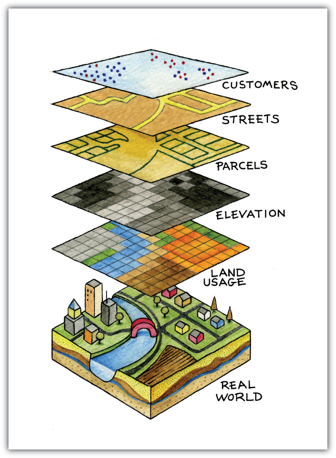
Create a feature column – essentially a regular non-spatial column

3

Create a geometry column containing an sfc object

4

sfc = geometry + spatial metadata

5

sfg = raw geometries

Simple feature collection with 4 features and 1 field
Geometry type: POINT
Dimension:     XY
Bounding box:  xmin: 1 ymin: 1 xmax: 2 ymax: 2
CRS:           NA
  feature    geometry
1       1 POINT (1 1)
2       2 POINT (1 2)
3       1 POINT (2 2)
4       2 POINT (2 1)

2.3 Coordinate reference systems

• All spatial data need to have a coordinate reference system (CRS) that locates the coordinates on the planet
• The geodetic specifics are mostly not necessary, but it’s always good to know a basic distinction
  • Geodetic CRS
    • Uses angular units (degrees) because they are based on a spheroid
    • Usually good for global or national scale visualizations
    • Example: WGS84 (World Geodetic System)
  • Projected CRS
    • Uses metric units (meters) because they are based on a projected model of the earth
    • Usually good for local or regional high-precision spatial analysis and visualization
    • Example: UTM (Universal Transversal Mercator)

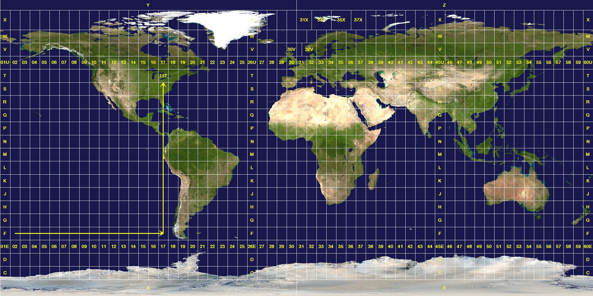
UTM (Universal Transversal Mercator) - a projected coordinate system. Each zone is a CRS.

2.4 EPSG codes

• CRS can be referenced using numeric identifiers called EPSG codes
  • EPSG database: https://epsg.io/, e.g. EPSG code 4326: https://epsg.io/4326

Some common CRS

Name	EPSG code	Area	Geodetic?	Use
World Geodetic System 1984 (WGS84)	4326	World	Yes	Basic geographic coordinates, common usage in GPS systems
WGS 84 / Pseudo-Mercator	3857	World	No	Google Maps, OpenStreetMap, general web mapping
UTM zone 32N	25832	Central Europe	No	Spatial analysis and measuring in Central Europe
LAEA Europe	3035	Europe	No	Multi-purpose CRS developed by the EU

2.5 CRS in R

• How do we work with CRS in R?
  • Convert to an sf dataframe: st_as_sf(..., crs = 4326)
  • Assign a CRS to an existing sf dataframe: st_crs(...) <- 4326 or st_set_crs(…, 4326)
  • Transform an existing CRS to a new CRS: st_transform(..., 4326)

2.6 Handling the Guerry dataset

• Let us take a look back at data_guerry and how to handle it as a spatial dataframe
• Guerry::gfrance85 comes as an sp dataframe, that’s a bit old so we have to convert it
• The dataset also comes with an invalid CRS, so we need to fix it

data_guerry <- Guerry::gfrance85 %>%
  st_as_sf() %>%
  as_tibble() %>%
  st_as_sf(crs = 27572) %>%
  mutate(Region = case_match(
    Region,
    "C" ~ "Central",
    "E" ~ "East",
    "N" ~ "North",
    "S" ~ "South",
    "W" ~ "West"
  )) %>%
  select(-c("COUNT", "dept", "AVE_ID_GEO", "CODE_DEPT")) %>% # drop columns
  select(Region:Department, all_of(names(variable_names))) # select columns

1

Guerry::gfrance85 comes as an sp object and it has no CRS information

2

…, so we convert it to an sf dataframe

3

Also convert it to a tibble to make it look nicer

4

Finally, convert it back to sf and set the CRS to 25572 (which is the native CRS of the Guerry data)

5

Here, we change the region coding that can be used for spatial aggregation

2.7 Spatial operations

• For mapping the Guerry data, a nice addition is to perform spatial aggregation to compare the data across geographical levels
• Spatial operations like spatial aggregations are one of the main advantages of spatial over regular data
• In Guerry, we have two levels: Departments (smaller) and regions (larger)
• In the following chunk we perform spatial aggregation outside of the server function

data_guerry_region <- data_guerry %>%
    group_by(Region) %>%
    summarise(across(
        .cols = all_of(names(variable_names)),
        function(x) {
            if (cur_column() %in% c("Area", "Pop1831")) {
                sum(x)
            } else {
                mean(x)
            }
        }
    ))

1

Define a group variable (Region)

2

Aggregate Guerry variables and geometries by their grouping variable Region. Features are summed or averaged while geometries are merged.

2.8 Guerry as spatial data

• Question: What can we say about the Guerry dataset in terms of spatial information?

data_guerry["Literacy"]

Simple feature collection with 85 features and 1 field
Geometry type: MULTIPOLYGON
Dimension:     XY
Bounding box:  xmin: 47680 ymin: 1703258 xmax: 1031401 ymax: 2677441
Projected CRS: NTF (Paris) / Lambert zone II
# A tibble: 85 × 2
   Literacy                                                             geometry
      <int>                                                   <MULTIPOLYGON [m]>
 1       37 (((801150 2092615, 800669 2093190, 800688 2095430, 800780 2095795, …
 2       51 (((729326 2521619, 729320 2521230, 729280 2518544, 728751 2517520, …
 3       13 (((710830 2137350, 711746 2136617, 712430 2135212, 712070 2134132, …
 4       46 (((882701 1920024, 882408 1920733, 881778 1921200, 881526 1922332, …
 5       69 (((886504 1922890, 885733 1922978, 885479 1923276, 883061 1925266, …
 6       27 (((747008 1925789, 746630 1925762, 745723 1925138, 744216 1925236, …
 7       67 (((818893 2514767, 818614 2514515, 817900 2514467, 817327 2514945, …
 8       18 (((509103 1747787, 508820 1747513, 508154 1747093, 505861 1746627, …
 9       59 (((775400 2345600, 775068 2345397, 773587 2345177, 772940 2344780, …
10       34 (((626230 1810121, 626269 1810496, 627494 1811321, 627681 1812424, …
# ℹ 75 more rows

2.9 Exercises

Exercise 1

Extract the sfc object from the Guerry dataset. What is the difference between sf and sfc?

Tip

Consult the documentation of st_geometry()

Solution

st_geometry(data_guerry)

sf objects are dataframes containing of one or more non-spatial feature columns and a geometry column containing an sfc object

sfc objects are representations of geospatial geometries. They contain all relevant spatial metadata but no contextual feature data

Exercise 2

Extract the fifth sfg object of the sfc object from exercise 1. What is the difference between the two?

Tip

Objects of class sfc behave like lists and can be subset in the same fashion

Solution

geom <- st_geometry(data_guerry)
geom[[1]]

sfg objects contain raw geometries consisting only of coordinates and a geometric topology (i.e. how to connect coordinates to make a polygon)

sfc objects have spatial metadata including the CRS which makes it possible to where the coordinates are located on the planet

Exercise 3

data_guerry currently consists of multi polygons. How can we convert these polygons to point geometries? Explore the function reference of the sf package and find functions (multiple answers possible) that can convert polygons to points in some way.

Tip

A search for “point” can give you the most obvious functions to fulfill the task, but there’s more!

Solution

st_point_on_surface(data_guerry) returns a point that is guaranteed to be on the polygon

st_centroid(data_guerry) returns the geometrical center of the polygon

st_cast(data_guerry, "POINT") or st_cast(data_guerry, "MULTIPOINT")

All of them return a warning! Why might that be?

st_sample(data_guerry, size = rep(1, nrow(data_guerry)))

Doesn’t return a warning, but is random and drops all features

Exercise 4

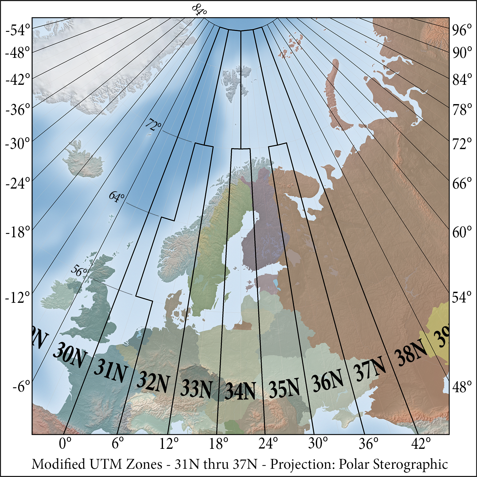
Currently, the Guerry dataframe has the CRS “NTF (Paris) / Lambert zone II”, which is already a good choice. What other CRS could be a good choice for accurate mapping in France?

Tip

Remember the UTM coordinate system! Scroll back up to see the UTM zones.

Solution

While there are many CRS that might be a good choice, one solution that we addressed in this workshop are UTM zones! Taking a look at the figure of UTM zones we can see that UTM zone 31N almost entirely covers the area of France.

Exercise 5

Transform the Guerry dataframe to your new CRS from exercise 4.

Tip

Remember you can visit https://epsg.io/ to look up EPSG codes.

Solution

Using the search function on epsg.io we can determine that the EPSG code to transform the Guerry dataset from Lambert zone II to UTM zone 31N is one of 23031, 25831 or 32631.

  st_transform(data_guerry, 23031)

3 Interactive maps using Leaflet

• R offers many solutions to mapping, some more advanced than others

  • ggplot2 supports spatial data with functions like geom_sf, coord_sf and custom ones like stars::geom_stars
  • tmap is a comprehensive framework for high-quality thematic mapping
  • cartography and mapsf incorporate cartography principles to move R closer to dedicated mapping software
  • leaflet interfaces the Leaflet JavaScript library to create interactive map visualizations

3.1 Integrate Leaflet in Shiny

• Leaflet in Shiny works just like any other type of visualization, we need:
  • A UI output: leaflet::leafletOutput()
  • A rendering function: leaflet::renderLeaflet()
• In our app, we add a geographic explorer of the Guerry dataset

tabItem(
  tabName = "tab_map",
  fluidRow(
    column(
      width = 12,
      box(
        id = "tab_map_box",
        status = "primary",
        headerBorder = FALSE,
        collapsible = FALSE,
        width = 12,
        leaflet::leafletOutput("tab_map_map", height = "800px", width = "100%")
      ) # end box
    ) # end column
  ) # end fluidRow
) # end tabItem

1

Create a new tab called tab_map

2

Add a fluid row containing a column and a box covering the entire page

3

Add a UI output that will hold the leaflet map. It covers the entire width and 800 pixels in height.

3.2 Leaflet workhorse

• The leaflet package is centered around the workhorse leaflet() which creates an empty map canvas
• Each additional function can be piped into and adds an additional mapping component (similar to ggplot2)
  • addProviderTiles() adds a base map, in this case we use four base maps that can be chosen from
  • addLayersControl() adds a button that lets you switch between map layers
  • setView() sets the center and zoom level of the initial map view

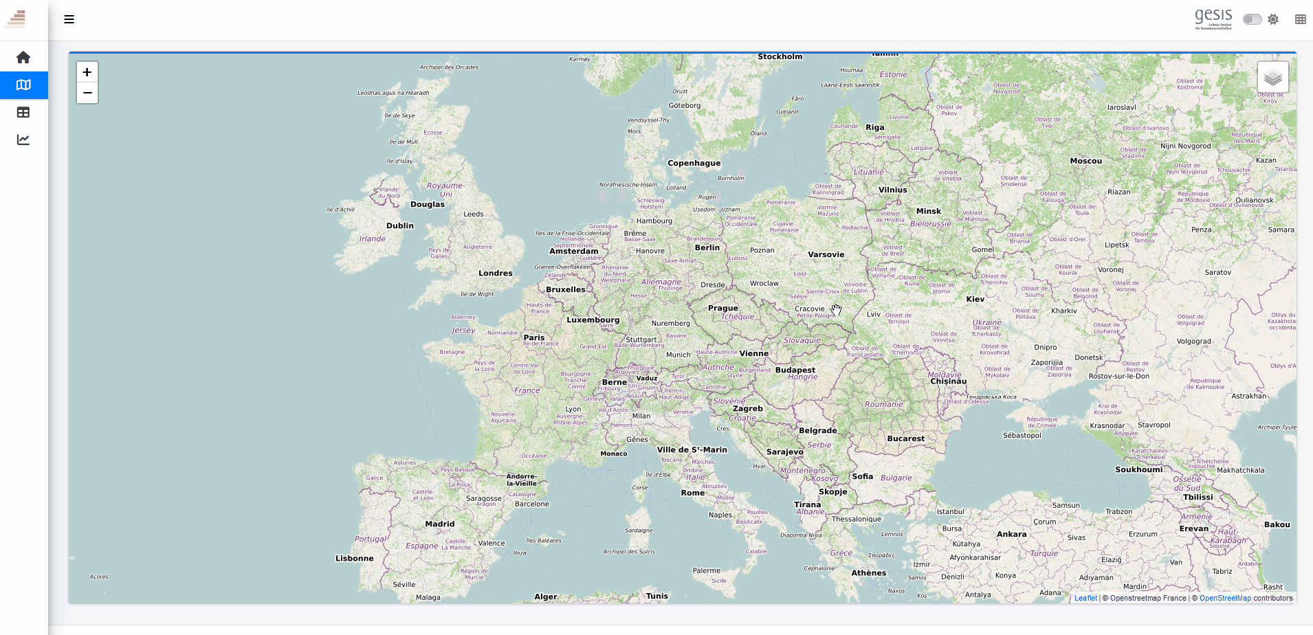
output$tab_map_map <- leaflet::renderLeaflet({
        leaflet() %>%
            addProviderTiles("OpenStreetMap.France", group = "OSM") %>%
            addProviderTiles("OpenTopoMap", group = "OTM") %>%
            addProviderTiles("Stamen.TonerLite", group = "Stamen Toner") %>%
            addProviderTiles("GeoportailFrance.orthos", group = "Orthophotos") %>%
            addLayersControl(baseGroups = c("OSM", "OTM",
                                                                            "Stamen Toner", "Orthophotos")) %>%
            setView(lng = 3, lat = 47, zoom = 5)
})

1

Fill the output tab_map_map with a leaflet map using renderLeaflet

2

Add an empty map using the power horse leaflet()

3

Add multiple basemaps: OpenStreetMap, OpenTopoMap, Stamen and ortho photos from the French geo portal

4

Add a button to control which of the basemaps to show

5

Set the initial center of the map and the zoom level

3.3 Full code

Full code including an empty map

library(shiny)
library(htmltools)
library(bs4Dash)
library(fresh)
library(waiter)
library(shinyWidgets)
library(Guerry)
library(sf)
library(tidyr)
library(dplyr)
library(RColorBrewer)
library(viridis)
library(leaflet)
library(plotly)
library(ggplot2)
library(GGally)
library(datawizard)
library(parameters)
library(performance)
library(modelsummary)

# 1 Data preparation ----

## Load & clean data ----
variable_names <- list(
  Crime_pers = "Crime against persons",  
  Crime_prop =  "Crime against property",  
  Literacy = "Literacy",  
  Donations = "Donations to the poor",  
  Infants = "Illegitimate births",  
  Suicides = "Suicides",  
  Wealth = "Tax / capita",  
  Commerce = "Commerce & Industry",  
  Clergy = "Clergy",  
  Crime_parents = "Crime against parents",  
  Infanticide = "Infanticides",  
  Donation_clergy = "Donations to the clergy",  
  Lottery = "Wager on Royal Lottery",  
  Desertion = "Military desertion",  
  Instruction = "Instruction",  
  Prostitutes = "Prostitutes",  
  Distance = "Distance to paris",  
  Area = "Area",  
  Pop1831 = "Population"
)

variable_desc <- list(
  Crime_pers = list(
    title = "Crime against persons",
    desc = as.character(p(tags$b("Crime against persons:"), "Population per crime against persons", hr(), helpText("Source: Table A2 in Guerry (1833). Compte général, 1825-1830"))),
    lgd = "Pop. per crime",
    unit = ""
  ),
  Crime_prop = list(
    title = "Crime against property",
    desc = as.character(p(tags$b("Crime against property:"), "Population per crime against property", hr(), helpText("Source: Compte général, 1825-1830"))),
    lgd = "Pop. per crime",
    unit = ""
  ),
  Literacy = list(
    title = "Literacy",
    desc = as.character(p(tags$b("Percent Read & Write:"), "Percent of military conscripts who can read and write", hr(), helpText("Source: Table A2 in Guerry (1833)"))),
    lgd = "Literacy",
    unit = " %"
  ),
  Donations = list(
    title = "Donations to the poor",
    desc = as.character(p(tags$b("Donations to the poor"), hr(), helpText("Source: Table A2 in Guerry (1833). Bulletin des lois"))),
    lgd = "Donations",
    unit = ""
  ),
  Infants = list(
    title = "Illegitimate births",
    desc = as.character(p(tags$b("Population per illegitimate birth"), hr(), helpText("Source: Table A2 in Guerry (1833). Bureau des Longitudes, 1817-1821"))),
    lgd = "Pop. per birth",
    unit = ""
  ),
  Suicides = list(
    title = "Suicides",
    desc = as.character(p(tags$b("Population per suicide"), hr(), helpText("Source: Table A2 in Guerry (1833). Compte général, 1827-1830"))),
    lgd = "Pop. per suicide",
    unit = ""
  ),
  Wealth = list(
    title = "Tax / capita",
    desc = as.character(p(tags$b("Per capita tax on personal property:"), "A ranked index based on taxes on personal and movable property per inhabitant", hr(), helpText("Source: Table A1 in Guerry (1833)"))),
    lgd = "Tax / capita",
    unit = ""
  ),
  Commerce = list(
    title = "Commerce & Industry",
    desc = as.character(p(tags$b("Commerce & Industry:"), "Commerce and Industry, measured by the rank of the number of patents / population", hr(), helpText("Source: Table A1 in Guerry (1833)"))),
    lgd = "Patents / capita",
    unit = ""
  ),
  Clergy = list(
    title = "Clergy",
    desc = as.character(p(tags$b("Distribution of clergy:"), "Distribution of clergy, measured by the rank of the number of Catholic priests in active service / population", hr(), helpText("Source: Table A1 in Guerry (1833). Almanach officiel du clergy, 1829"))),
    lgd = "Priests / capita",
    unit = ""
  ),
  Crime_parents = list(
    title = "Crime against parents",
    desc = as.character(p(tags$b("Crime against parents:"), "Crimes against parents, measured by the rank of the ratio of crimes against parents to all crimes \u2013 Average for the years 1825-1830", hr(), helpText("Source: Table A1 in Guerry (1833). Compte général"))),
    lgd = "Share of crimes",
    unit = " %"
  ),
  Infanticide = list(
    title = "Infanticides",
    desc = as.character(p(tags$b("Infanticides per capita:"), "Ranked ratio of number of infanticides to population \u2013 Average for the years 1825-1830", hr(), helpText("Source: Table A1 in Guerry (1833). Compte général"))),
    lgd = "Infanticides / capita",
    unit = ""
  ),
  Donation_clergy = list(
    title = "Donations to the clergy",
    desc = as.character(p(tags$b("Donations to the clergy:"), "Ranked ratios of the number of bequests and donations inter vivios to population \u2013 Average for the years 1815-1824", hr(), helpText("Source: Table A1 in Guerry (1833). Bull. des lois, ordunn. d’autorisation"))),
    lgd = "Donations / capita",
    unit = ""
  ),
  Lottery = list(
    title = "Wager on Royal Lottery",
    desc = as.character(p(tags$b("Per capita wager on Royal Lottery:"), "Ranked ratio of the proceeds bet on the royal lottery to population \u2013 Average for the years 1822-1826", hr(), helpText("Source: Table A1 in Guerry (1833). Compte rendu par le ministre des finances"))),
    lgd = "Wager / capita",
    unit = ""
  ),
  Desertion = list(
    title = "Military desertion",
    desc = as.character(p(tags$b("Military desertion:"), "Military disertion, ratio of the number of young soldiers accused of desertion to the force of the military contingent, minus the deficit produced by the insufficiency of available billets\u2013 Average of the years 1825-1827", hr(), helpText("Source: Table A1 in Guerry (1833). Compte du ministère du guerre, 1829 état V"))),
    lgd = "No. of desertions",
    unit = ""
  ),
  Instruction = list(
    title = "Instruction",
    desc = as.character(p(tags$b("Instruction:"), "Ranks recorded from Guerry's map of Instruction. Note: this is inversely related to literacy (as defined here)")),
    lgd = "Instruction",
    unit = ""
  ),
  Prostitutes = list(
    title = "Prostitutes",
    desc = as.character(p(tags$b("Prostitutes in Paris:"), "Number of prostitutes registered in Paris from 1816 to 1834, classified by the department of their birth", hr(), helpText("Source: Parent-Duchatelet (1836), De la prostitution en Paris"))),
    lgd = "No. of prostitutes",
    unit = ""
  ),
  Distance = list(
    title = "Distance to paris",
    desc = as.character(p(tags$b("Distance to Paris (km):"), "Distance of each department centroid to the centroid of the Seine (Paris)", hr(), helpText("Source: Calculated from department centroids"))),
    lgd = "Distance",
    unit = " km"
  ),
  Area = list(
    title = "Area",
    desc = as.character(p(tags$b("Area (1000 km\u00b2)"), hr(), helpText("Source: Angeville (1836)"))),
    lgd = "Area",
    unit = " km\u00b2"
  ),
  Pop1831 = list(
    title = "Population",
    desc = as.character(p(tags$b("Population in 1831, in 1000s"), hr(), helpText("Source: Taken from Angeville (1836), Essai sur la Statistique de la Population français"))),
    lgd = "Population (in 1000s)",
    unit = ""
  )
)

data_guerry <- Guerry::gfrance85 %>%
  st_as_sf() %>%
  as_tibble() %>%
  st_as_sf(crs = 27572) %>%
  mutate(Region = case_match(
    Region,
    "C" ~ "Central",
    "E" ~ "East",
    "N" ~ "North",
    "S" ~ "South",
    "W" ~ "West"
  )) %>%
  select(-c("COUNT", "dept", "AVE_ID_GEO", "CODE_DEPT")) %>%
  select(Region:Department, all_of(names(variable_names)))



## Prep data (Tab: Tabulate data) ----
data_guerry_tabulate <- data_guerry %>% 
  st_drop_geometry() %>% 
  mutate(across(.cols = all_of(names(variable_names)), round, 2))


## Prep data (Tab: Map data) ----
data_guerry_region <- data_guerry %>%
  group_by(Region) %>%
  summarise(across(
    .cols = all_of(names(variable_names)),
    function(x) {
      if (cur_column() %in% c("Area", "Pop1831")) {
        sum(x)
      } else {
        mean(x)
      }
    }
  ))

## Prepare palettes ----
## Used for mapping
pals <- list(
  Sequential = RColorBrewer::brewer.pal.info %>%
    filter(category %in% "seq") %>%
    row.names(),
  Viridis = c("Magma", "Inferno", "Plasma", "Viridis",
              "Cividis", "Rocket", "Mako", "Turbo")
)

## Prepare modebar clean-up ----
## Used for modelling
plotly_buttons <- c(
  "sendDataToCloud", "zoom2d", "select2d", "lasso2d", "autoScale2d",
  "hoverClosestCartesian", "hoverCompareCartesian", "resetScale2d"
)




# 3 UI ----

ui <- dashboardPage(
  title = "The Guerry Dashboard",
  ## 3.1 Header ----
  header = dashboardHeader(
    title = tagList(
      img(src = "../workshop-logo.png", width = 35, height = 35),
      span("The Guerry Dashboard", class = "brand-text")
    )
  ),
  ## 3.2 Sidebar ----
  sidebar = dashboardSidebar(
    id = "sidebar",
    sidebarMenu(
      id = "sidebarMenu",
      menuItem(tabName = "tab_intro", text = "Introduction", icon = icon("home")),
      menuItem(tabName = "tab_tabulate", text = "Tabulate data", icon = icon("table")),
      menuItem(tabName = "tab_model", text = "Model data", icon = icon("chart-line")),
      menuItem(tabName = "tab_map", text = "Map data", icon = icon("map")),
      flat = TRUE
    ),
    minified = TRUE,
    collapsed = TRUE,
    fixed = FALSE,
    skin = "light"
  ),
  ## 3.3 Body ----
  body = dashboardBody(
    tabItems(
      ### 3.1.1 Tab: Introduction ----
      tabItem(
        tabName = "tab_intro",
        jumbotron(
          title = "The Guerry Dashboard",
          lead = "A Shiny app to explore the classic Guerry dataset.",
          status = "info",
          btnName = NULL
        ),
        fluidRow(
          column(width = 1),
          column(
            width = 6,
            box(
              title = "About",
              status = "primary",
              width = 12,
              blockQuote(HTML("André-Michel Guerry was a French lawyer and
                          amateur statistician. Together with Adolphe
                          Quetelet he may be regarded as the founder of
                          moral statistics which led to the development
                          of criminology, sociology and ultimately,
                          modern social science. <br>— Wikipedia: <a href='https://en.wikipedia.org/wiki/Andr%C3%A9-Michel_Guerry'>André-Michel Guerry</a>"),
                         color = "primary"),
              p(HTML("Andre-Michel Guerry (1833) was the first to 
              systematically collect and analyze social data 
               on such things as crime, literacy and suicide 
               with the view to determining social laws and the 
               relations among these variables. The Guerry data 
               frame comprises a collection of 'moral variables' 
               (cf. <i><a href='https://en.wikipedia.org/wiki/Moral_statistics'>moral statistics</a></i>) 
               on the 86 departments of France around 1830. 
               A few additional variables have been added 
               from other sources. In total the data frame has 
               86 observations (the departments of France) on 23 variables <i>(Source: <code>?Guerry</code>)</i>. 
               In this app, we aim to explore Guerry’s data
                using spatial exploration and regression modelling.")),
              hr(),
              accordion(
                id = "accord",
                accordionItem(
                  title = "References",
                  status = "primary",
                  solidHeader = FALSE,
                  "The following sources are referenced in this app:",
                  tags$ul(
                    class = "list-style: none",
                    style = "margin-left: -30px;",
                    p("Angeville, A. (1836). Essai sur la Statistique de la Population française Paris: F. Doufour."),
                    p("Guerry, A.-M. (1833). Essai sur la statistique morale de la France Paris: Crochard. English translation: Hugh P. Whitt and Victor W. Reinking, Lewiston, N.Y. : Edwin Mellen Press, 2002."),
                    p("Parent-Duchatelet, A. (1836). De la prostitution dans la ville de Paris, 3rd ed, 1857, p. 32, 36"),
                    p("Palsky, G. (2008). Connections and exchanges in European thematic cartography. The case of 19th century choropleth maps. Belgeo 3-4, 413-426.")
                  )
                ),
                accordionItem(
                  title = "Details",
                  status = "primary",
                  solidHeader = FALSE,
                  p("This app was created as part of a Shiny workshop held in July 2023"),
                  p("Last update: June 2023"),
                  p("Further information about the data can be found",
                    a("here.", href = "https://www.datavis.ca/gallery/guerry/guerrydat.html"))
                )
              )
            )
          ),
          column(
            width = 4,
            box(
              title = "André Michel Guerry",
              status = "primary",
              width = 12,
              tags$img(src = "../guerry.jpg", width = "100%"),
              p("Source: Palsky (2008)")
            )
          )
        )
      ),
      ### 3.3.2 Tab: Tabulate data ----
      tabItem(
        tabName = "tab_tabulate",
        fluidRow(
          #### Inputs(s) ----
          pickerInput(
            "tab_tabulate_select",
            label = "Filter variables",
            choices = setNames(names(variable_names), variable_names),
            options = pickerOptions(
              actionsBox = TRUE,
              windowPadding = c(30, 0, 0, 0),
              liveSearch = TRUE,
              selectedTextFormat = "count",
              countSelectedText = "{0} variables selected",
              noneSelectedText = "No filters applied"
            ),
            inline = TRUE,
            multiple = TRUE
          )
        ),
        hr(),
        #### Output(s) (Data table) ----
        DT::dataTableOutput("tab_tabulate_table")
      ),
      ### 3.3.3 Tab: Model data ----
      tabItem(
        tabName = "tab_model",
        fluidRow(
          column(
            width = 6,
            #### Inputs(s) ----
            box(
              width = 12,
              title = "Select variables",
              status = "primary",
              shinyWidgets::pickerInput(
                "model_x",
                label = "Select a dependent variable",
                choices = setNames(names(variable_names), variable_names),
                options = shinyWidgets::pickerOptions(liveSearch = TRUE),
                selected = "Literacy"
              ),
              shinyWidgets::pickerInput(
                "model_y",
                label = "Select independent variables",
                choices = setNames(names(variable_names), variable_names),
                options = shinyWidgets::pickerOptions(
                  actionsBox = TRUE,
                  liveSearch = TRUE,
                  selectedTextFormat = "count",
                  countSelectedText = "{0} variables selected",
                  noneSelectedText = "No variables selected"
                ),
                multiple = TRUE,
                selected = "Commerce"
              ),
              shinyWidgets::prettyCheckbox(
                "model_std",
                label = "Standardize variables?",
                value = TRUE,
                status = "primary",
                shape = "curve"
              ),
              hr(),
              actionButton(
                "refresh",
                label = "Apply changes",
                icon = icon("refresh"),
                flat = TRUE
              )
            ),
            #### Outputs(s) ----
            tabBox(
              status = "primary",
              type = "tabs",
              title = "Model analysis",
              side = "right",
              width = 12,
              ##### Tabpanel: Coefficient plot ----
              tabPanel(
                title = "Plot: Coefficients",
                plotly::plotlyOutput("coefficientplot")
              ),
              ##### Tabpanel: Scatterplot ----
              tabPanel(
                title = "Plot: Scatterplot",
                plotly::plotlyOutput("scatterplot")
              ),
              ##### Tabpanel: Table: Regression ----
              tabPanel(
                title = "Table: Model",
                htmlOutput("tableregression")
              )
            )
          ),
          column(
            width = 6,
            ##### Box: Pair diagramm ----
            box(
              width = 12,
              title = "Pair diagram",
              status = "primary",
              plotly::plotlyOutput("pairplot")
            ),
            ##### TabBox: Model diagnostics ----
            tabBox(
              status = "primary",
              type = "tabs",
              title = "Model diagnostics",
              width = 12,
              side = "right",
              tabPanel(
                title = "Normality",
                plotly::plotlyOutput("normality")
              ),
              tabPanel(
                title = "Outliers",
                plotly::plotlyOutput("outliers")
              ),
              tabPanel(
                title = "Heteroskedasticity",
                plotly::plotlyOutput("heteroskedasticity")
              )
            )
          )
        )
      ),
      ### 3.3.4 Tab: Map data ----
      tabItem(
        tabName = "tab_map", # must correspond to related menuItem name
        fluidRow(
          column(
            #### Output(s) ----
            width = 8,
            box(
              id = "tab_map_box",
              status = "primary",
              headerBorder = FALSE,
              collapsible = FALSE,
              width = 12,
              leaflet::leafletOutput("tab_map_map", height = "800px", width = "100%")
            ) # end box
          ) # end column
        ) # end fluidRow
      ) # end tabItem
    ) # end tabItems
  ),
  
  ## 3.4 Footer (bottom)----
  footer = dashboardFooter(
    left = span(
      "This dashboard was created by Jonas Lieth and Paul Bauer. Find the source code",
      a("here.", href = "https://github.com/paulcbauer/shiny_workshop/tree/main/shinyapps/guerry"),
      "It is based on data from the",
      a("Guerry R package.", href = "https://cran.r-project.org/web/packages/Guerry/index.html")
    )
  ),
  ## 3.5 Controlbar (top)----
  controlbar = dashboardControlbar(
    div(class = "p-3", skinSelector()),
    skin = "light"
  )  
)



# 4 Server ----

server <- function(input, output, session) {
  
  ## 4.1 Tabulate data ----
  ### Variable selection ----
  tab <- reactive({
    var <- input$tab_tabulate_select
    data_table <- data_guerry_tabulate
    
    if (!is.null(var)) {
      data_table <- data_table[, var]
    }
    
    data_table
  })
  
  
  ### Create table----
  dt <- reactive({
    tab <- tab()
    ridx <- ifelse("Department" %in% names(tab), 3, 1)
    DT::datatable(
      tab,
      class = "hover",
      extensions = c("Buttons"),
      selection = "none",
      filter = list(position = "top", clear = FALSE),
      style = "bootstrap4",
      rownames = FALSE,
      options = list(
        dom = "Brtip",
        deferRender = TRUE,
        scroller = TRUE,
        buttons = list(
          list(extend = "copy", text = "Copy to clipboard"),
          list(extend = "pdf", text = "Save as PDF"),
          list(extend = "csv", text = "Save as CSV"),
          list(extend = "excel", text = "Save as JSON", action = DT::JS("
          function (e, dt, button, config) {
            var data = dt.buttons.exportData();
  
            $.fn.dataTable.fileSave(
              new Blob([JSON.stringify(data)]),
              'Shiny dashboard.json'
            );
          }
        "))
        )
      )
    )
  })
  
  ### Render table----
  output$tab_tabulate_table <- DT::renderDataTable(dt(), server = FALSE)
  
  
  
  ## 4.2 Model data ----
  ### Define & estimate model ----
  mparams <- reactive({
    x <- input$model_x
    y <- input$model_y
    dt <- sf::st_drop_geometry(data_guerry)[c(x, y)]
    dt_labels <- sf::st_drop_geometry(data_guerry)[c("Department", "Region")]
    if (input$model_std) dt <- datawizard::standardise(dt)
    form <- as.formula(paste(x, "~", paste(y, collapse = " + ")))
    mod <- lm(form, data = dt)
    
    list(
      x = x,
      y = y,
      data = dt,
      data_labels = dt_labels,
      model = mod
    )
  }) %>%
    bindEvent(input$refresh, ignoreNULL = FALSE)
  
  ### Pair diagram ----
  output$pairplot <- plotly::renderPlotly({
    params <- mparams()
    dt <- params$data
    dt_labels <- params$data_labels
    p <- GGally::ggpairs(
      params$data,
      axisLabels = "none",
      lower = list(
        continuous = function(data, mapping, ...) {
          ggplot(data, mapping) +
            suppressWarnings(geom_point(
              aes(text = paste0(
                "Department: ", 
                dt_labels[["Department"]],
                "<br>Region: ", 
                dt_labels[["Region"]])),
              color = "black"
            ))
        }
      )
    )
    if (isTRUE(input$dark_mode)) p <- p +
      dark_theme_gray() +
      theme(plot.background = element_rect(fill = "#343a40"))
    ggplotly(p) %>%
      config(modeBarButtonsToRemove = plotly_buttons,
             displaylogo = FALSE)
  })
  
  ### Plot: Coefficientplot ----
  output$coefficientplot <- renderPlotly({
    params <- mparams()
    dt <- params$data
    x <- params$x
    y <- params$y
    
    
    p <- plot(parameters::model_parameters(params$model))
    
    if (isTRUE(input$dark_mode)) p <- p +
      geom_point(color = "white") +
      dark_theme_gray() +
      theme(plot.background = element_rect(fill = "#343a40"))
    ggplotly(p) %>%
      config(modeBarButtonsToRemove = plotly_buttons,
             displaylogo = FALSE)
  })
  
  ### Plot: Scatterplot ----
  output$scatterplot <- renderPlotly({
    params <- mparams()
    dt <- params$data
    dt_labels <- params$data_labels
    x <- params$x 
    y <- params$y
    
    
    if (length(y) == 1) {
      p <- ggplot(params$data, 
                  aes(x = .data[[params$x]], 
                      y = .data[[params$y]])) +
        geom_point(aes(text = paste0("Department: ", 
                                     dt_labels[["Department"]],
                                     "<br>Region: ", 
                                     dt_labels[["Region"]])),
                   color = "black") +
        geom_smooth() + 
        geom_smooth(method='lm') +
        theme_light()
    } else {
      p <- ggplot() +
        theme_void() +
        annotate("text", 
                 label = "Cannot create scatterplot.\nMore than two variables selected.", 
                 x = 0, y = 0, 
                 size = 5, 
                 colour = "red",
                 hjust = 0.5,
                 vjust = 0.5) +
        xlab(NULL)
      
    }
    
    if (isTRUE(input$dark_mode)) p <- p +
      geom_point(color = "white") +
      dark_theme_gray() +
      theme(plot.background = element_rect(fill = "#343a40"))
    ggplotly(p) %>%
      config(modeBarButtonsToRemove = plotly_buttons,
             displaylogo = FALSE)
  })
  
  ### Table: Regression ----
  output$tableregression <- renderUI({
    params <- mparams()
    HTML(modelsummary(
      dvnames(list(params$model)),
      gof_omit = "AIC|BIC|Log|Adj|RMSE"
    ))
  })
  
  ### Plot: Normality residuals ----
  output$normality <- renderPlotly({
    params <- mparams()
    p <- plot(performance::check_normality(params$model))
    if (isTRUE(input$dark_mode)) p <- p +
      dark_theme_gray() +
      theme(plot.background = element_rect(fill = "#343a40"))
    ggplotly(p) %>%
      config(modeBarButtonsToRemove = plotly_buttons,
             displaylogo = FALSE)
  })
  
  ### Plot: Outliers ----
  output$outliers <- renderPlotly({
    params <- mparams()
    p <- plot(performance::check_outliers(params$model), show_labels = FALSE)
    if (isTRUE(input$dark_mode)) p <- p +
      dark_theme_gray() +
      theme(plot.background = element_rect(fill = "#343a40"))
    p$labels$x <- "Leverage"
    ggplotly(p) %>%
      config(modeBarButtonsToRemove = plotly_buttons,
             displaylogo = FALSE)
  })
  
  ### Plot: Heteroskedasticity ----
  output$heteroskedasticity <- renderPlotly({
    params <- mparams()
    p <- plot(performance::check_heteroskedasticity(params$model))
    if (isTRUE(input$dark_mode)) p <- p +
      dark_theme_gray() +
      theme(plot.background = element_rect(fill = "#343a40"))
    p$labels$y <- "Sqrt. |Std. residuals|" # ggplotly doesn't support expressions
    ggplotly(p) %>%
      config(modeBarButtonsToRemove = plotly_buttons,
             displaylogo = FALSE)
  })
  
  
  ## 4.3 Map data ----
  output$tab_map_map <- leaflet::renderLeaflet({
    leaflet() %>%
      addProviderTiles("OpenStreetMap.France", group = "OSM") %>%
      addProviderTiles("OpenTopoMap", group = "OTM") %>%
      addProviderTiles("Stamen.TonerLite", group = "Stamen Toner") %>%
      addProviderTiles("GeoportailFrance.orthos", group = "Orthophotos") %>%
      addLayersControl(baseGroups = c("OSM", "OTM",
                                      "Stamen Toner", "Orthophotos")) %>%
      setView(lng = 3, lat = 47, zoom = 5)
  })
}

shinyApp(ui, server)

4 Add data

• Currently, we only show a background, but do not map the Guerry data
• Adding data works using layer functions, for example:
  • addMarkers() adds point data
  • addPolylines() adds line data
  • addPolygons() adds polygon data
  • addRasterImage() adds raster data
  • addLegend() adds a legend

4.1 Specifics of Leaflet mapping

• Variables are passed using formulas (i.e. instead of data_guerry$Literacy, we write ~Literacy)
• Leaflet by default only supports WGS84 (EPSG:4326) as CRS
• Palettes are applied using custom functions that are generated in function factories:
  • colorNumeric() maps continuous values
  • colorBin() bins continuous values evenly
  • colorQuantile() bins continuous values based on their quantiles
  • colorFactor() maps categorical values
• highlightOptions() adds a nice highlight effect when hovering over a polygon

output$tab_map_map <- leaflet::renderLeaflet({
    pal <- colorNumeric(palette = "Reds", domain = NULL)
    
    leaflet(data = st_transform(data_guerry, 4326)) %>%
        addProviderTiles("OpenStreetMap.France") %>%
        setView(lng = 3, lat = 47, zoom = 5) %>%
        addPolygons(
            fillColor = ~params$pal(Literacy),
            fillOpacity = 0.7,
            weight = 1,
            color = "black",
            opacity = 0.5,
            highlightOptions = highlightOptions(
                weight = 2,
                color = "black",
                opacity = 0.5,
                fillOpacity = 1,
                bringToFront = TRUE,
                sendToBack = TRUE
            )
        ) %>%
        addLegend(
            position = "bottomright",
            pal = pal,
            values = ~Literacy,
            opacity = 0.9,
            title = "Literacy",
            labFormat = labelFormat(suffix = " %")
        )
})

1

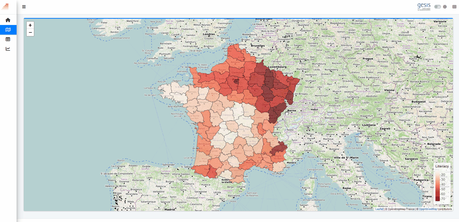
Determine the color palette for mapping. Here, we want to map continious values in red. The output is a function called pal() which we can use later on.

2

Create an empty map. Add spatial data. Note that leaflet by default only accepts spatial data with EPSG:4326. For anything else, consult leaflet::leafletCRS(), but don’t expect to understand much of what’s going on.

3

Add a basemap of OpenStreetMap France

4

Set the center and zoom level of the initial view

5

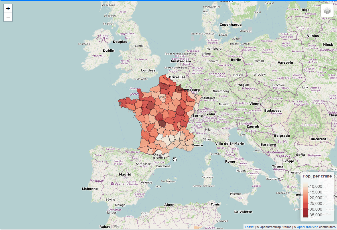
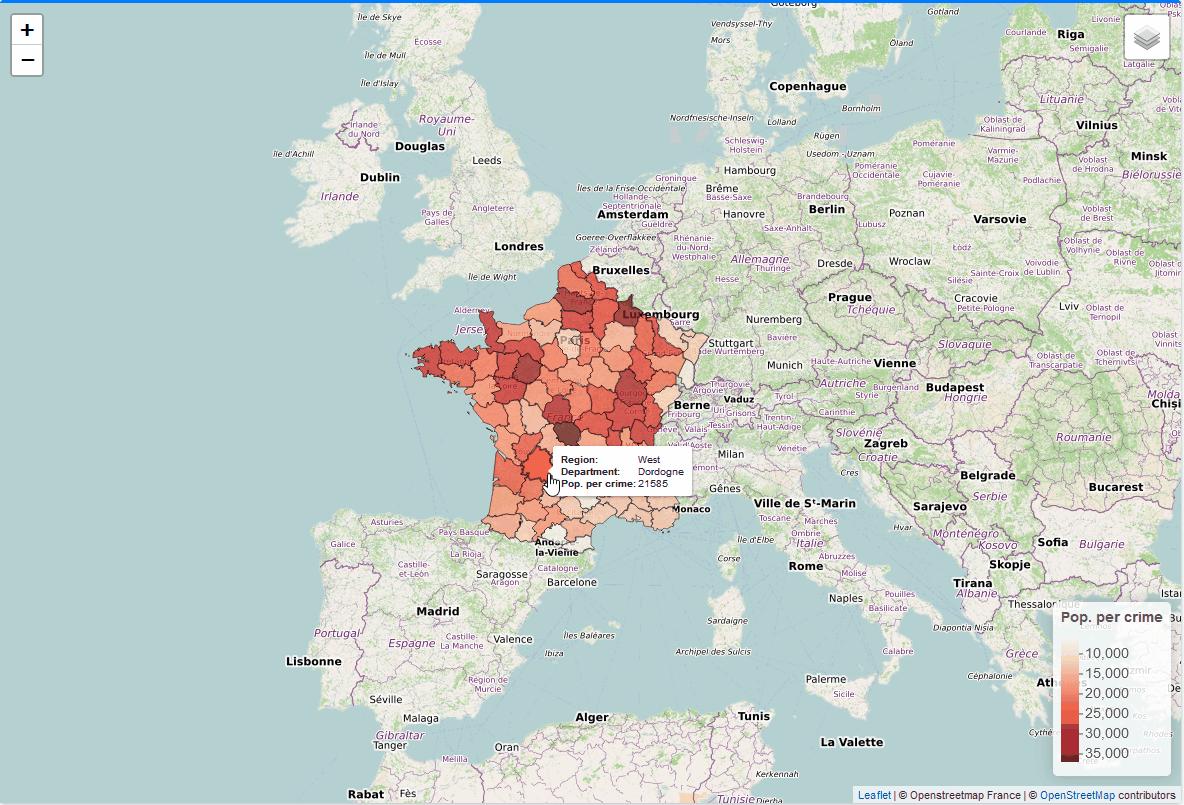
The addPolygons() function adds polygons to the leaflet map

6

fillColor determines how the polygons should be colored. We pass a formula that contains a call to our generated function pal() (see point 2) that maps colors to the Literacy variable.

7

We can add additional parameters that control the appearance of the map, e.g. opacity, color or line thickness (weight).

8

highlightOptions() allows you to add a nice highlight effect when hovering over the polygons

9

Using addLegend() we add a legend to the bottom right of the Leaflet map

10

addLegend() accepts values in the same way as addPolygons(): pal accepts the generated palette function and values accepts a formula containing the column name in the input dataset.

11

Finally, labelFormat() allows you to change the formatting of the legend label, e.g. if you need to specify whether a number is a percentage, meters or something else

4.2 Full code

Full code including a simple Leaflet map

library(shiny)
library(htmltools)
library(bs4Dash)
library(fresh)
library(waiter)
library(shinyWidgets)
library(Guerry)
library(sf)
library(tidyr)
library(dplyr)
library(RColorBrewer)
library(viridis)
library(leaflet)
library(plotly)
library(ggplot2)
library(GGally)
library(datawizard)
library(parameters)
library(performance)
library(modelsummary)

# 1 Data preparation ----

## Load & clean data ----
variable_names <- list(
  Crime_pers = "Crime against persons",  
  Crime_prop =  "Crime against property",  
  Literacy = "Literacy",  
  Donations = "Donations to the poor",  
  Infants = "Illegitimate births",  
  Suicides = "Suicides",  
  Wealth = "Tax / capita",  
  Commerce = "Commerce & Industry",  
  Clergy = "Clergy",  
  Crime_parents = "Crime against parents",  
  Infanticide = "Infanticides",  
  Donation_clergy = "Donations to the clergy",  
  Lottery = "Wager on Royal Lottery",  
  Desertion = "Military desertion",  
  Instruction = "Instruction",  
  Prostitutes = "Prostitutes",  
  Distance = "Distance to paris",  
  Area = "Area",  
  Pop1831 = "Population"
)

variable_desc <- list(
  Crime_pers = list(
    title = "Crime against persons",
    desc = as.character(p(tags$b("Crime against persons:"), "Population per crime against persons", hr(), helpText("Source: Table A2 in Guerry (1833). Compte général, 1825-1830"))),
    lgd = "Pop. per crime",
    unit = ""
  ),
  Crime_prop = list(
    title = "Crime against property",
    desc = as.character(p(tags$b("Crime against property:"), "Population per crime against property", hr(), helpText("Source: Compte général, 1825-1830"))),
    lgd = "Pop. per crime",
    unit = ""
  ),
  Literacy = list(
    title = "Literacy",
    desc = as.character(p(tags$b("Percent Read & Write:"), "Percent of military conscripts who can read and write", hr(), helpText("Source: Table A2 in Guerry (1833)"))),
    lgd = "Literacy",
    unit = " %"
  ),
  Donations = list(
    title = "Donations to the poor",
    desc = as.character(p(tags$b("Donations to the poor"), hr(), helpText("Source: Table A2 in Guerry (1833). Bulletin des lois"))),
    lgd = "Donations",
    unit = ""
  ),
  Infants = list(
    title = "Illegitimate births",
    desc = as.character(p(tags$b("Population per illegitimate birth"), hr(), helpText("Source: Table A2 in Guerry (1833). Bureau des Longitudes, 1817-1821"))),
    lgd = "Pop. per birth",
    unit = ""
  ),
  Suicides = list(
    title = "Suicides",
    desc = as.character(p(tags$b("Population per suicide"), hr(), helpText("Source: Table A2 in Guerry (1833). Compte général, 1827-1830"))),
    lgd = "Pop. per suicide",
    unit = ""
  ),
  Wealth = list(
    title = "Tax / capita",
    desc = as.character(p(tags$b("Per capita tax on personal property:"), "A ranked index based on taxes on personal and movable property per inhabitant", hr(), helpText("Source: Table A1 in Guerry (1833)"))),
    lgd = "Tax / capita",
    unit = ""
  ),
  Commerce = list(
    title = "Commerce & Industry",
    desc = as.character(p(tags$b("Commerce & Industry:"), "Commerce and Industry, measured by the rank of the number of patents / population", hr(), helpText("Source: Table A1 in Guerry (1833)"))),
    lgd = "Patents / capita",
    unit = ""
  ),
  Clergy = list(
    title = "Clergy",
    desc = as.character(p(tags$b("Distribution of clergy:"), "Distribution of clergy, measured by the rank of the number of Catholic priests in active service / population", hr(), helpText("Source: Table A1 in Guerry (1833). Almanach officiel du clergy, 1829"))),
    lgd = "Priests / capita",
    unit = ""
  ),
  Crime_parents = list(
    title = "Crime against parents",
    desc = as.character(p(tags$b("Crime against parents:"), "Crimes against parents, measured by the rank of the ratio of crimes against parents to all crimes \u2013 Average for the years 1825-1830", hr(), helpText("Source: Table A1 in Guerry (1833). Compte général"))),
    lgd = "Share of crimes",
    unit = " %"
  ),
  Infanticide = list(
    title = "Infanticides",
    desc = as.character(p(tags$b("Infanticides per capita:"), "Ranked ratio of number of infanticides to population \u2013 Average for the years 1825-1830", hr(), helpText("Source: Table A1 in Guerry (1833). Compte général"))),
    lgd = "Infanticides / capita",
    unit = ""
  ),
  Donation_clergy = list(
    title = "Donations to the clergy",
    desc = as.character(p(tags$b("Donations to the clergy:"), "Ranked ratios of the number of bequests and donations inter vivios to population \u2013 Average for the years 1815-1824", hr(), helpText("Source: Table A1 in Guerry (1833). Bull. des lois, ordunn. d’autorisation"))),
    lgd = "Donations / capita",
    unit = ""
  ),
  Lottery = list(
    title = "Wager on Royal Lottery",
    desc = as.character(p(tags$b("Per capita wager on Royal Lottery:"), "Ranked ratio of the proceeds bet on the royal lottery to population \u2013 Average for the years 1822-1826", hr(), helpText("Source: Table A1 in Guerry (1833). Compte rendu par le ministre des finances"))),
    lgd = "Wager / capita",
    unit = ""
  ),
  Desertion = list(
    title = "Military desertion",
    desc = as.character(p(tags$b("Military desertion:"), "Military disertion, ratio of the number of young soldiers accused of desertion to the force of the military contingent, minus the deficit produced by the insufficiency of available billets\u2013 Average of the years 1825-1827", hr(), helpText("Source: Table A1 in Guerry (1833). Compte du ministère du guerre, 1829 état V"))),
    lgd = "No. of desertions",
    unit = ""
  ),
  Instruction = list(
    title = "Instruction",
    desc = as.character(p(tags$b("Instruction:"), "Ranks recorded from Guerry's map of Instruction. Note: this is inversely related to literacy (as defined here)")),
    lgd = "Instruction",
    unit = ""
  ),
  Prostitutes = list(
    title = "Prostitutes",
    desc = as.character(p(tags$b("Prostitutes in Paris:"), "Number of prostitutes registered in Paris from 1816 to 1834, classified by the department of their birth", hr(), helpText("Source: Parent-Duchatelet (1836), De la prostitution en Paris"))),
    lgd = "No. of prostitutes",
    unit = ""
  ),
  Distance = list(
    title = "Distance to paris",
    desc = as.character(p(tags$b("Distance to Paris (km):"), "Distance of each department centroid to the centroid of the Seine (Paris)", hr(), helpText("Source: Calculated from department centroids"))),
    lgd = "Distance",
    unit = " km"
  ),
  Area = list(
    title = "Area",
    desc = as.character(p(tags$b("Area (1000 km\u00b2)"), hr(), helpText("Source: Angeville (1836)"))),
    lgd = "Area",
    unit = " km\u00b2"
  ),
  Pop1831 = list(
    title = "Population",
    desc = as.character(p(tags$b("Population in 1831, in 1000s"), hr(), helpText("Source: Taken from Angeville (1836), Essai sur la Statistique de la Population français"))),
    lgd = "Population (in 1000s)",
    unit = ""
  )
)

data_guerry <- Guerry::gfrance85 %>%
  st_as_sf() %>%
  as_tibble() %>%
  st_as_sf(crs = 27572) %>%
  mutate(Region = case_match(
    Region,
    "C" ~ "Central",
    "E" ~ "East",
    "N" ~ "North",
    "S" ~ "South",
    "W" ~ "West"
  )) %>%
  select(-c("COUNT", "dept", "AVE_ID_GEO", "CODE_DEPT")) %>%
  select(Region:Department, all_of(names(variable_names)))



## Prep data (Tab: Tabulate data) ----
data_guerry_tabulate <- data_guerry %>% 
  st_drop_geometry() %>% 
  mutate(across(.cols = all_of(names(variable_names)), round, 2))


## Prep data (Tab: Map data) ----
data_guerry_region <- data_guerry %>%
  group_by(Region) %>%
  summarise(across(
    .cols = all_of(names(variable_names)),
    function(x) {
      if (cur_column() %in% c("Area", "Pop1831")) {
        sum(x)
      } else {
        mean(x)
      }
    }
  ))

## Prepare palettes ----
## Used for mapping
pals <- list(
  Sequential = RColorBrewer::brewer.pal.info %>%
    filter(category %in% "seq") %>%
    row.names(),
  Viridis = c("Magma", "Inferno", "Plasma", "Viridis",
              "Cividis", "Rocket", "Mako", "Turbo")
)

## Prepare modebar clean-up ----
## Used for modelling
plotly_buttons <- c(
  "sendDataToCloud", "zoom2d", "select2d", "lasso2d", "autoScale2d",
  "hoverClosestCartesian", "hoverCompareCartesian", "resetScale2d"
)




# 3 UI ----

ui <- dashboardPage(
  title = "The Guerry Dashboard",
  ## 3.1 Header ----
  header = dashboardHeader(
    title = tagList(
      img(src = "../workshop-logo.png", width = 35, height = 35),
      span("The Guerry Dashboard", class = "brand-text")
    )
  ),
  ## 3.2 Sidebar ----
  sidebar = dashboardSidebar(
    id = "sidebar",
    sidebarMenu(
      id = "sidebarMenu",
      menuItem(tabName = "tab_intro", text = "Introduction", icon = icon("home")),
      menuItem(tabName = "tab_tabulate", text = "Tabulate data", icon = icon("table")),
      menuItem(tabName = "tab_model", text = "Model data", icon = icon("chart-line")),
      menuItem(tabName = "tab_map", text = "Map data", icon = icon("map")),
      flat = TRUE
    ),
    minified = TRUE,
    collapsed = TRUE,
    fixed = FALSE,
    skin = "light"
  ),
  ## 3.3 Body ----
  body = dashboardBody(
    tabItems(
      ### 3.1.1 Tab: Introduction ----
      tabItem(
        tabName = "tab_intro",
        jumbotron(
          title = "The Guerry Dashboard",
          lead = "A Shiny app to explore the classic Guerry dataset.",
          status = "info",
          btnName = NULL
        ),
        fluidRow(
          column(width = 1),
          column(
            width = 6,
            box(
              title = "About",
              status = "primary",
              width = 12,
              blockQuote(HTML("André-Michel Guerry was a French lawyer and
                          amateur statistician. Together with Adolphe
                          Quetelet he may be regarded as the founder of
                          moral statistics which led to the development
                          of criminology, sociology and ultimately,
                          modern social science. <br>— Wikipedia: <a href='https://en.wikipedia.org/wiki/Andr%C3%A9-Michel_Guerry'>André-Michel Guerry</a>"),
                         color = "primary"),
              p(HTML("Andre-Michel Guerry (1833) was the first to 
              systematically collect and analyze social data 
               on such things as crime, literacy and suicide 
               with the view to determining social laws and the 
               relations among these variables. The Guerry data 
               frame comprises a collection of 'moral variables' 
               (cf. <i><a href='https://en.wikipedia.org/wiki/Moral_statistics'>moral statistics</a></i>) 
               on the 86 departments of France around 1830. 
               A few additional variables have been added 
               from other sources. In total the data frame has 
               86 observations (the departments of France) on 23 variables <i>(Source: <code>?Guerry</code>)</i>. 
               In this app, we aim to explore Guerry’s data
                using spatial exploration and regression modelling.")),
              hr(),
              accordion(
                id = "accord",
                accordionItem(
                  title = "References",
                  status = "primary",
                  solidHeader = FALSE,
                  "The following sources are referenced in this app:",
                  tags$ul(
                    class = "list-style: none",
                    style = "margin-left: -30px;",
                    p("Angeville, A. (1836). Essai sur la Statistique de la Population française Paris: F. Doufour."),
                    p("Guerry, A.-M. (1833). Essai sur la statistique morale de la France Paris: Crochard. English translation: Hugh P. Whitt and Victor W. Reinking, Lewiston, N.Y. : Edwin Mellen Press, 2002."),
                    p("Parent-Duchatelet, A. (1836). De la prostitution dans la ville de Paris, 3rd ed, 1857, p. 32, 36"),
                    p("Palsky, G. (2008). Connections and exchanges in European thematic cartography. The case of 19th century choropleth maps. Belgeo 3-4, 413-426.")
                  )
                ),
                accordionItem(
                  title = "Details",
                  status = "primary",
                  solidHeader = FALSE,
                  p("This app was created as part of a Shiny workshop held in July 2023"),
                  p("Last update: June 2023"),
                  p("Further information about the data can be found",
                    a("here.", href = "https://www.datavis.ca/gallery/guerry/guerrydat.html"))
                )
              )
            )
          ),
          column(
            width = 4,
            box(
              title = "André Michel Guerry",
              status = "primary",
              width = 12,
              tags$img(src = "../guerry.jpg", width = "100%"),
              p("Source: Palsky (2008)")
            )
          )
        )
      ),
      ### 3.3.2 Tab: Tabulate data ----
      tabItem(
        tabName = "tab_tabulate",
        fluidRow(
          #### Inputs(s) ----
          pickerInput(
            "tab_tabulate_select",
            label = "Filter variables",
            choices = setNames(names(variable_names), variable_names),
            options = pickerOptions(
              actionsBox = TRUE,
              windowPadding = c(30, 0, 0, 0),
              liveSearch = TRUE,
              selectedTextFormat = "count",
              countSelectedText = "{0} variables selected",
              noneSelectedText = "No filters applied"
            ),
            inline = TRUE,
            multiple = TRUE
          )
        ),
        hr(),
        #### Output(s) (Data table) ----
        DT::dataTableOutput("tab_tabulate_table")
      ),
      ### 3.3.3 Tab: Model data ----
      tabItem(
        tabName = "tab_model",
        fluidRow(
          column(
            width = 6,
            #### Inputs(s) ----
            box(
              width = 12,
              title = "Select variables",
              status = "primary",
              shinyWidgets::pickerInput(
                "model_x",
                label = "Select a dependent variable",
                choices = setNames(names(variable_names), variable_names),
                options = shinyWidgets::pickerOptions(liveSearch = TRUE),
                selected = "Literacy"
              ),
              shinyWidgets::pickerInput(
                "model_y",
                label = "Select independent variables",
                choices = setNames(names(variable_names), variable_names),
                options = shinyWidgets::pickerOptions(
                  actionsBox = TRUE,
                  liveSearch = TRUE,
                  selectedTextFormat = "count",
                  countSelectedText = "{0} variables selected",
                  noneSelectedText = "No variables selected"
                ),
                multiple = TRUE,
                selected = "Commerce"
              ),
              shinyWidgets::prettyCheckbox(
                "model_std",
                label = "Standardize variables?",
                value = TRUE,
                status = "primary",
                shape = "curve"
              ),
              hr(),
              actionButton(
                "refresh",
                label = "Apply changes",
                icon = icon("refresh"),
                flat = TRUE
              )
            ),
            #### Outputs(s) ----
            tabBox(
              status = "primary",
              type = "tabs",
              title = "Model analysis",
              side = "right",
              width = 12,
              ##### Tabpanel: Coefficient plot ----
              tabPanel(
                title = "Plot: Coefficients",
                plotly::plotlyOutput("coefficientplot")
              ),
              ##### Tabpanel: Scatterplot ----
              tabPanel(
                title = "Plot: Scatterplot",
                plotly::plotlyOutput("scatterplot")
              ),
              ##### Tabpanel: Table: Regression ----
              tabPanel(
                title = "Table: Model",
                htmlOutput("tableregression")
              )
            )
          ),
          column(
            width = 6,
            ##### Box: Pair diagramm ----
            box(
              width = 12,
              title = "Pair diagram",
              status = "primary",
              plotly::plotlyOutput("pairplot")
            ),
            ##### TabBox: Model diagnostics ----
            tabBox(
              status = "primary",
              type = "tabs",
              title = "Model diagnostics",
              width = 12,
              side = "right",
              tabPanel(
                title = "Normality",
                plotly::plotlyOutput("normality")
              ),
              tabPanel(
                title = "Outliers",
                plotly::plotlyOutput("outliers")
              ),
              tabPanel(
                title = "Heteroskedasticity",
                plotly::plotlyOutput("heteroskedasticity")
              )
            )
          )
        )
      ),
      ### 3.3.4 Tab: Map data ----
      tabItem(
        tabName = "tab_map", # must correspond to related menuItem name
        fluidRow(
          column(
            #### Output(s) ----
            width = 8,
            box(
              id = "tab_map_box",
              status = "primary",
              headerBorder = FALSE,
              collapsible = FALSE,
              width = 12,
              leaflet::leafletOutput("tab_map_map", height = "800px", width = "100%")
            ) # end box
          ) # end column
        ) # end fluidRow
      ) # end tabItem
    ) # end tabItems
  ),
  
  ## 3.4 Footer (bottom)----
  footer = dashboardFooter(
    left = span(
      "This dashboard was created by Jonas Lieth and Paul Bauer. Find the source code",
      a("here.", href = "https://github.com/paulcbauer/shiny_workshop/tree/main/shinyapps/guerry"),
      "It is based on data from the",
      a("Guerry R package.", href = "https://cran.r-project.org/web/packages/Guerry/index.html")
    )
  ),
  ## 3.5 Controlbar (top)----
  controlbar = dashboardControlbar(
    div(class = "p-3", skinSelector()),
    skin = "light"
  )  
)



# 4 Server ----

server <- function(input, output, session) {
  
  ## 4.1 Tabulate data ----
  ### Variable selection ----
  tab <- reactive({
    var <- input$tab_tabulate_select
    data_table <- data_guerry_tabulate
    
    if (!is.null(var)) {
      data_table <- data_table[, var]
    }
    
    data_table
  })
  
  
  ### Create table----
  dt <- reactive({
    tab <- tab()
    ridx <- ifelse("Department" %in% names(tab), 3, 1)
    DT::datatable(
      tab,
      class = "hover",
      extensions = c("Buttons"),
      selection = "none",
      filter = list(position = "top", clear = FALSE),
      style = "bootstrap4",
      rownames = FALSE,
      options = list(
        dom = "Brtip",
        deferRender = TRUE,
        scroller = TRUE,
        buttons = list(
          list(extend = "copy", text = "Copy to clipboard"),
          list(extend = "pdf", text = "Save as PDF"),
          list(extend = "csv", text = "Save as CSV"),
          list(extend = "excel", text = "Save as JSON", action = DT::JS("
          function (e, dt, button, config) {
            var data = dt.buttons.exportData();
  
            $.fn.dataTable.fileSave(
              new Blob([JSON.stringify(data)]),
              'Shiny dashboard.json'
            );
          }
        "))
        )
      )
    )
  })
  
  ### Render table----
  output$tab_tabulate_table <- DT::renderDataTable(dt(), server = FALSE)
  
  
  
  ## 4.2 Model data ----
  ### Define & estimate model ----
  mparams <- reactive({
    x <- input$model_x
    y <- input$model_y
    dt <- sf::st_drop_geometry(data_guerry)[c(x, y)]
    dt_labels <- sf::st_drop_geometry(data_guerry)[c("Department", "Region")]
    if (input$model_std) dt <- datawizard::standardise(dt)
    form <- as.formula(paste(x, "~", paste(y, collapse = " + ")))
    mod <- lm(form, data = dt)
    
    list(
      x = x,
      y = y,
      data = dt,
      data_labels = dt_labels,
      model = mod
    )
  }) %>%
    bindEvent(input$refresh, ignoreNULL = FALSE)
  
  ### Pair diagram ----
  output$pairplot <- plotly::renderPlotly({
    params <- mparams()
    dt <- params$data
    dt_labels <- params$data_labels
    p <- GGally::ggpairs(
      params$data,
      axisLabels = "none",
      lower = list(
        continuous = function(data, mapping, ...) {
          ggplot(data, mapping) +
            suppressWarnings(geom_point(
              aes(text = paste0(
                "Department: ", 
                dt_labels[["Department"]],
                "<br>Region: ", 
                dt_labels[["Region"]])),
              color = "black"
            ))
        }
      )
    )
    if (isTRUE(input$dark_mode)) p <- p +
      dark_theme_gray() +
      theme(plot.background = element_rect(fill = "#343a40"))
    ggplotly(p) %>%
      config(modeBarButtonsToRemove = plotly_buttons,
             displaylogo = FALSE)
  })
  
  ### Plot: Coefficientplot ----
  output$coefficientplot <- renderPlotly({
    params <- mparams()
    dt <- params$data
    x <- params$x
    y <- params$y
    
    
    p <- plot(parameters::model_parameters(params$model))
    
    if (isTRUE(input$dark_mode)) p <- p +
      geom_point(color = "white") +
      dark_theme_gray() +
      theme(plot.background = element_rect(fill = "#343a40"))
    ggplotly(p) %>%
      config(modeBarButtonsToRemove = plotly_buttons,
             displaylogo = FALSE)
  })
  
  ### Plot: Scatterplot ----
  output$scatterplot <- renderPlotly({
    params <- mparams()
    dt <- params$data
    dt_labels <- params$data_labels
    x <- params$x 
    y <- params$y
    
    
    if (length(y) == 1) {
      p <- ggplot(params$data, 
                  aes(x = .data[[params$x]], 
                      y = .data[[params$y]])) +
        geom_point(aes(text = paste0("Department: ", 
                                     dt_labels[["Department"]],
                                     "<br>Region: ", 
                                     dt_labels[["Region"]])),
                   color = "black") +
        geom_smooth() + 
        geom_smooth(method='lm') +
        theme_light()
    } else {
      p <- ggplot() +
        theme_void() +
        annotate("text", 
                 label = "Cannot create scatterplot.\nMore than two variables selected.", 
                 x = 0, y = 0, 
                 size = 5, 
                 colour = "red",
                 hjust = 0.5,
                 vjust = 0.5) +
        xlab(NULL)
      
    }
    
    if (isTRUE(input$dark_mode)) p <- p +
      geom_point(color = "white") +
      dark_theme_gray() +
      theme(plot.background = element_rect(fill = "#343a40"))
    ggplotly(p) %>%
      config(modeBarButtonsToRemove = plotly_buttons,
             displaylogo = FALSE)
  })
  
  ### Table: Regression ----
  output$tableregression <- renderUI({
    params <- mparams()
    HTML(modelsummary(
      dvnames(list(params$model)),
      gof_omit = "AIC|BIC|Log|Adj|RMSE"
    ))
  })
  
  ### Plot: Normality residuals ----
  output$normality <- renderPlotly({
    params <- mparams()
    p <- plot(performance::check_normality(params$model))
    if (isTRUE(input$dark_mode)) p <- p +
      dark_theme_gray() +
      theme(plot.background = element_rect(fill = "#343a40"))
    ggplotly(p) %>%
      config(modeBarButtonsToRemove = plotly_buttons,
             displaylogo = FALSE)
  })
  
  ### Plot: Outliers ----
  output$outliers <- renderPlotly({
    params <- mparams()
    p <- plot(performance::check_outliers(params$model), show_labels = FALSE)
    if (isTRUE(input$dark_mode)) p <- p +
      dark_theme_gray() +
      theme(plot.background = element_rect(fill = "#343a40"))
    p$labels$x <- "Leverage"
    ggplotly(p) %>%
      config(modeBarButtonsToRemove = plotly_buttons,
             displaylogo = FALSE)
  })
  
  ### Plot: Heteroskedasticity ----
  output$heteroskedasticity <- renderPlotly({
    params <- mparams()
    p <- plot(performance::check_heteroskedasticity(params$model))
    if (isTRUE(input$dark_mode)) p <- p +
      dark_theme_gray() +
      theme(plot.background = element_rect(fill = "#343a40"))
    p$labels$y <- "Sqrt. |Std. residuals|" # ggplotly doesn't support expressions
    ggplotly(p) %>%
      config(modeBarButtonsToRemove = plotly_buttons,
             displaylogo = FALSE)
  })
  
  
  ## 4.3 Map data ----
  # Render leaflet for the first time
  output$tab_map_map <- leaflet::renderLeaflet({
    pal <- colorNumeric(palette = "Reds", domain = NULL)
    
    leaflet(data = st_transform(data_guerry, 4326)) %>%
      addProviderTiles("OpenStreetMap.France", group = "OSM") %>%
      addProviderTiles("OpenTopoMap", group = "OTM") %>%
      addProviderTiles("Stamen.TonerLite", group = "Stamen Toner") %>%
      addProviderTiles("GeoportailFrance.orthos", group = "Orthophotos") %>%
      addLayersControl(baseGroups = c("OSM", "OTM", "Stamen Toner", "Orthophotos")) %>%
      setView(lng = 3, lat = 47, zoom = 5) %>%
      addPolygons(
        fillColor = ~pal(Literacy),
        fillOpacity = 0.7,
        weight = 1,
        color = "black",
        opacity = 0.5,
        highlightOptions = highlightOptions(
          weight = 2,
          color = "black",
          opacity = 0.5,
          fillOpacity = 1,
          bringToFront = TRUE,
          sendToBack = TRUE
        )
      ) %>%
      addLegend(
        position = "bottomright",
        pal = pal,
        values = ~Literacy,
        opacity = 0.9,
        title = "Literacy",
        labFormat = labelFormat(suffix = " %")
      )
  })
}

shinyApp(ui, server)

4.3 Exercises

Exercise 1

Classify the mapped values into deciles (i.e., ten equally sized bins).

Tip

Consult the documentation of ?colorNumeric(). Particularly watch out for the other three color* functions.

Solution

Legend values can be binned using either the colorBin() or the colorQuantile() function. Since we want to map deciles, we need to use the colorQuantile() function and increase the number of bins to 10.

Instead of using colorNumeric() to create the palette function

pal <- colorNumeric(palette = "Reds", domain = NULL)

… we can exchange it with colorQuantile():

pal <- colorQuantile(palette = "Reds", domain = NULL, n = 10)

Exercise 2

Let the opacity of the polygons scale with the values of the Commerce variable in the Guerry dataset. Also add a label that shows the values of Literacy in the following form: “value: <literacy value here>”.

Tip

Remember that data columns can be specified using the ~ symbol! This also applies to entire function calls.

If you are not sure about how to control opacity and labels, consult ?addPolygons().

Solution

Using the Leaflet formulas, we can scale many arguments to the add* functions in any way we want. To scale the fill opacity using the Commerce variable, we can add fillOpacity = ~Commerce / 100. We divide by 100 to adjust the Commerce variable to the scale of opacity values (usually 0-1).

In the same way, we can provide hover labels

  leaflet(data = st_transform(data_guerry, 4326)) %>%
    addProviderTiles("OpenStreetMap.France", group = "OSM") %>%
    addProviderTiles("OpenTopoMap", group = "OTM") %>%
    addProviderTiles("Stamen.TonerLite", group = "Stamen Toner") %>%
    addProviderTiles("GeoportailFrance.orthos", group = "Orthophotos") %>%
    addLayersControl(baseGroups = c("OSM", "OTM", "Stamen Toner", "Orthophotos")) %>%
    setView(lng = 3, lat = 47, zoom = 5) %>%
    addPolygons(
      fillColor = ~pal(Literacy),
      fillOpacity = ~Commerce / 100,
      weight = 1,
      color = "black",
      opacity = 0.5,
      label = ~paste0("value: ", Literacy),
      highlightOptions = highlightOptions(
        weight = 2,
        color = "black",
        opacity = 0.5,
        fillOpacity = 1,
        bringToFront = TRUE,
        sendToBack = TRUE
      )
    ) %>%
    addLegend(
      position = "bottomright",
      pal = pal,
      values = ~Literacy,
      opacity = 0.9,
      title = "Literacy",
      labFormat = labelFormat(suffix = " %")
    )

1

Scale the fill opacity using the Commerce variable. Since opacity is measured using percentages and Commerce is scaled somewhere around values of 1-100, we need to rescale Commerce by dividing it with 100.

2

Within a formula expression, we can put any R expression. Thus, to combine values and text, we can just use paste0() on them.

Exercise 3

How could we go about adding a second line to the hover label that also shows the value for the Commerce variable? In other words, how can we add a hover label of the following form:

Literacy: <literacy value here>

Commerce: <commerce value here>

The solution does not have to be code, ideas are also welcome!

Tip

Regular R line breaks (\n) don’t work in Shiny. Why is that? What can we use instead (remember section 3 about HTML tags)?

Warning

Regular R line breaks don’t work, because Shiny apps are HTML documents. In section 3, we talked about HTML tags including the br() function producing the <br/> HTML tag. The code for a label with two lines could look something like this:

leaflet() %>%
  addPolygons(
    ..., # rest of the arguments
    label = ~lapply(paste0("Literacy: ", Literacy, br(), "Commerce: ", Commerce), HTML),
  )

Note: If we are dealing with character vectors containing HTML, we need to wrap them in a call to HTML() so R knows it’s dealing with HTML!

5 Add reactivity

• Similar to chapter 5 on visualization, reactivity is the key to making maps in Shiny
• Similar to chapter 5, reactivity is arguably the most complex part of app development!

5.1 Reactive UI

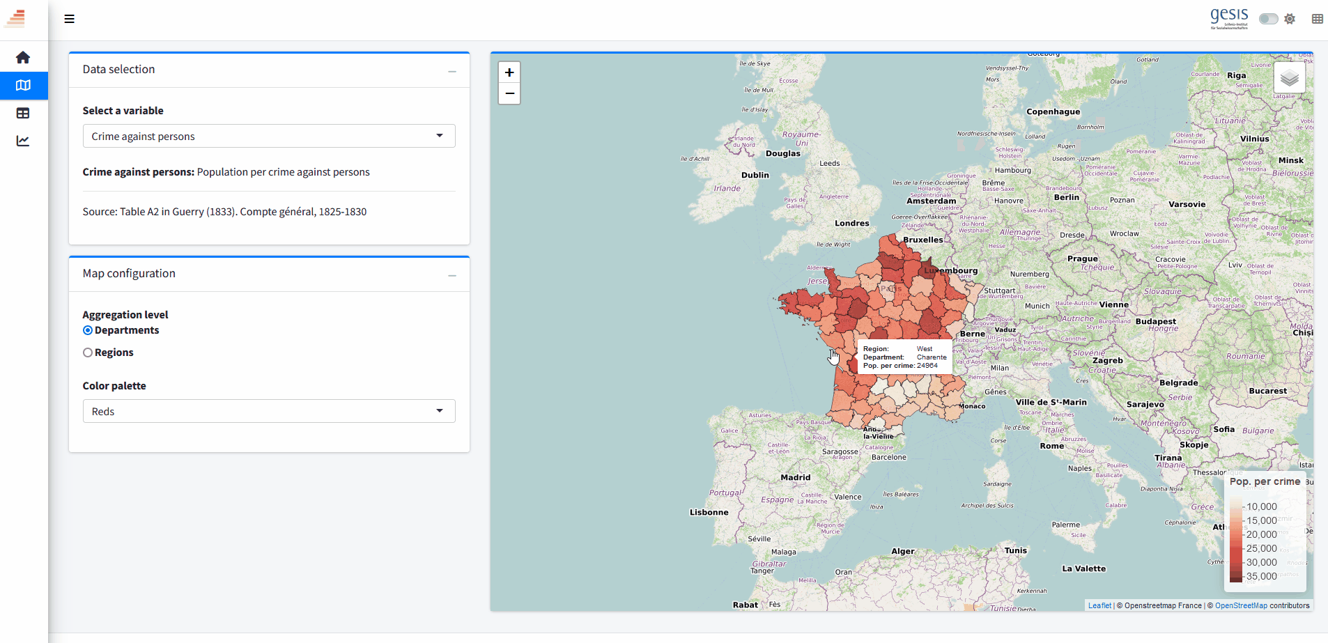
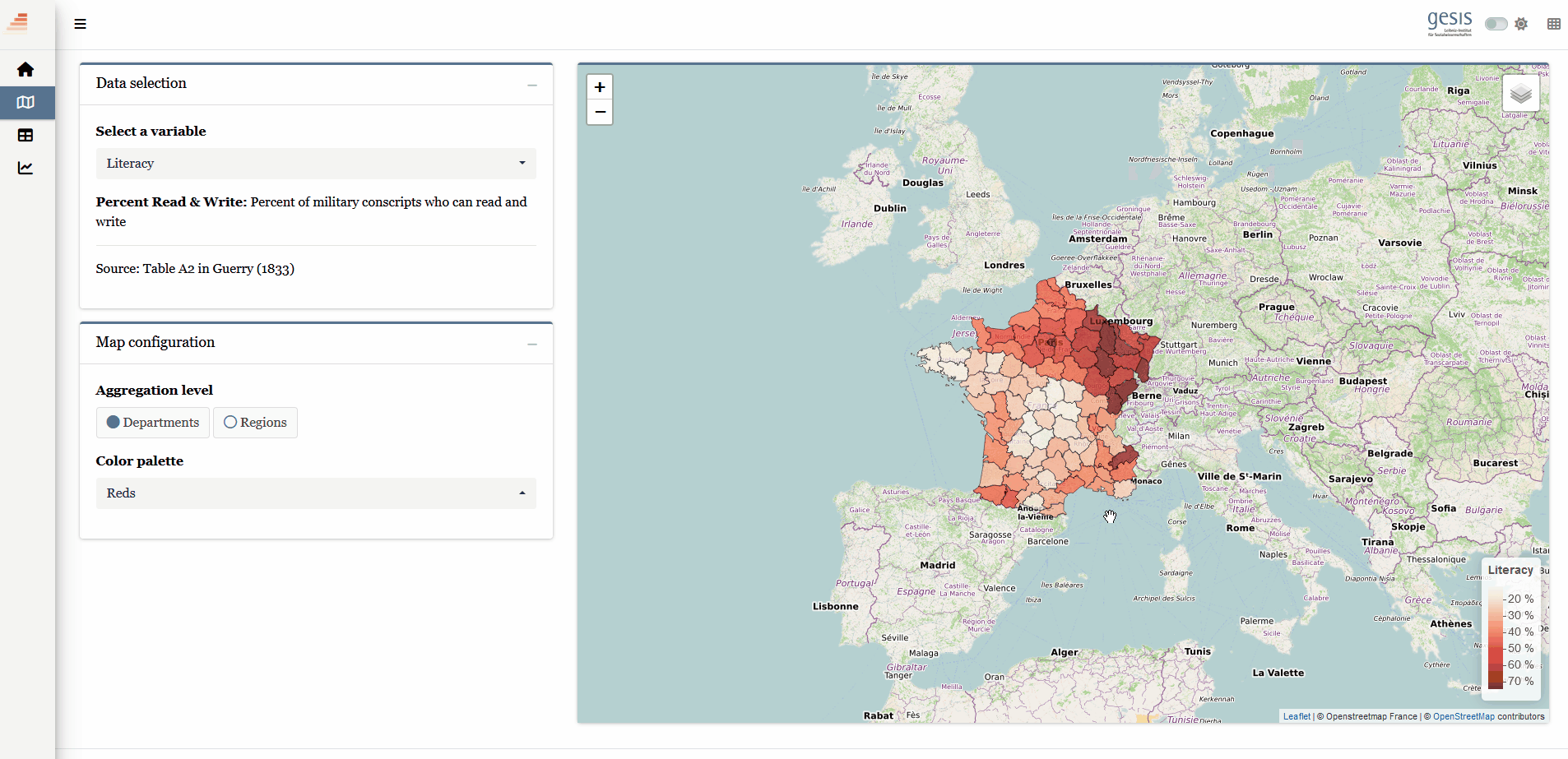
• In our app, we add three reactive components:
  • selectInput() to select a variable to map
  • radioButtons() to select an aggregation level, departments or regions
  • selectInput() to select a color palette
• Additionally, one new UI output (tab_map_desc) is added that describes the selected variable

# Define selectable palettes: All sequential palettes + viridis
pals <- list(
  Sequential = RColorBrewer::brewer.pal.info %>%
    filter(category %in% "seq") %>%
    row.names(),
  Viridis = c("Magma", "Inferno", "Plasma", "Viridis",
              "Cividis", "Rocket", "Mako", "Turbo")
)

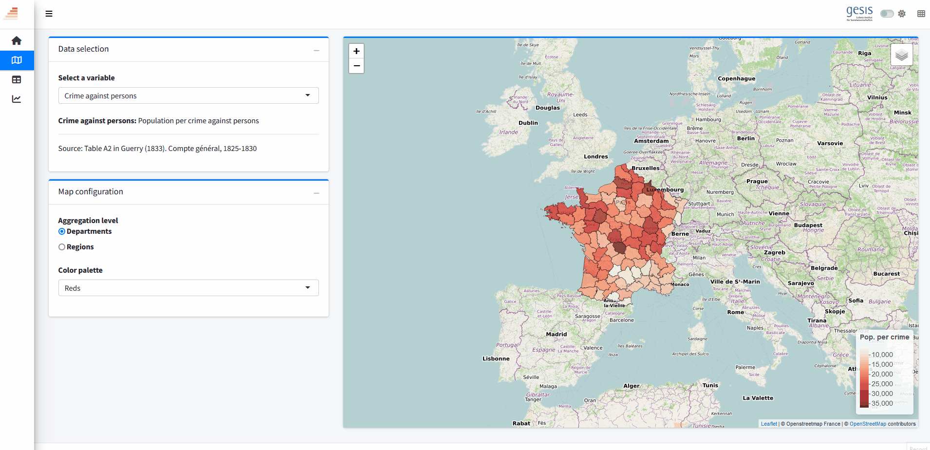
tabItem(
    tabName = "tab_map",
    fluidRow(
        column(
            width = 4,
            box(
                title = "Data selection",
                status = "primary",
                width = 12,
                selectInput(
                    "tab_map_select",
                    label = "Select a variable",
                    choices = setNames(variable_names, names(variable_names))
                )
            ),
            box(
                title = "Map configuration",
                status = "primary",
                width = 12,
                radioButtons(
                    "tab_map_aggr",
                    label = "Aggregation level",
                    choices = c("Departments", "Regions"),
                    selected = "Departments"
                ),
                selectInput(
                    "tab_map_pal",
                    label = "Color palette",
                    choices = pals,
                    selected = "Reds"
                ) # end input
            ) # end box
        ), # end column
        column(
            width = 8,
            box(
                id = "tab_map_box",
                status = "primary",
                headerBorder = FALSE,
                collapsible = FALSE,
                width = 12,
                leaflet::leafletOutput("tab_map_map", height = "800px", width = "100%")
            ) # end box
        ) # end column
    ) # end fluidRow
) # end tabItem

1

Previously, the map tab only consisted of one column with a box. Now we add another column that occupies 1/3 of the page where we add our UI inputs

2

Add a dropdown menu that selects a variable to map

3

Add a second box. Since both boxes have a width of 12

5.2 Server side

• In the server function, we have a lot to do:
  • Apply the selected aggregation level
  • Apply the selected palette
  • Change hard code to adaptive code

    # Select polygon based on aggregation level
    poly <- reactive({
        if (identical(input$tab_map_aggr, "Regions")) {
            data_guerry_region
        } else {
            data_guerry
        }
    })
    
    # Select palette based on input
    palette <- reactive({
        pal <- input$tab_map_pal
        if (pal %in% pals$Viridis) {
            pal <- viridis::viridis_pal(option = tolower(pal))(5)
        }
        pal
    })
    
    # Compile parameters for leaflet rendering
    params <- reactive({
        poly <- st_transform(poly(), 4326)
        pal <- palette()
        var <- input$tab_map_select

        values <- as.formula(paste0("~", var))
        pal <- colorNumeric(palette = pal, domain = NULL)

        list(
            poly = poly,
            var = var,
            pal = pal,
            values = values
        )
    })
    
    # Render leaflet for the first time
    output$tab_map_map <- leaflet::renderLeaflet({
        # Isolate call to params() to prevent render function to be executed
        # every time params() is invalidated. No dependency is made.
        params <- params()
        leaflet(data = params$poly) %>%
            addProviderTiles("OpenStreetMap.France", group = "OSM") %>%
            addProviderTiles("OpenTopoMap", group = "OTM") %>%
            addProviderTiles("Stamen.TonerLite", group = "Stamen Toner") %>%
            addProviderTiles("GeoportailFrance.orthos", group = "Orthophotos") %>%
            addLayersControl(baseGroups = c("OSM", "OTM",
                                                                            "Stamen Toner", "Orthophotos")) %>%
            setView(lng = 3, lat = 47, zoom = 5) %>%
            addPolygons(
                fillColor = as.formula(paste0("~params$pal(", params$var, ")")),
                fillOpacity = 0.7,
                weight = 1,
                color = "black",
                opacity = 0.5,
                highlightOptions = highlightOptions(
                    weight = 2,
                    color = "black",
                    opacity = 0.5,
                    fillOpacity = 1,
                    bringToFront = TRUE,
                    sendToBack = TRUE
                )
            ) %>%
            addLegend(
                position = "bottomright",
                pal = params$pal,
                values = params$values,
                opacity = 0.9
            )
    })

1

In a reactive expression called poly() we catch the selected aggregation level and decide whether to use the original data_guerry or the aggregated variant data_guerry_region.

2

In a reactive expression called palette() we catch the selected palette and match it with the available palette names.

3

We combine all inputs in a reactive expression called params() where we do the remaining data wrangling before the input data goes into leaflet mapping

4

Finally, we do the mapping and replace all previously hard-coded information with our new reactive data. This includes the input dataframe which is now simply params$poly, the fill color which is now a formula that is pasted together from the palette function and the selected variable and finally the palette and values required for the legend.

5.3 Full code

Full code including a reactive Leaflet map

library(shiny)
library(htmltools)
library(bs4Dash)
library(fresh)
library(waiter)
library(shinyWidgets)
library(Guerry)
library(sf)
library(tidyr)
library(dplyr)
library(RColorBrewer)
library(viridis)
library(leaflet)
library(plotly)
library(ggplot2)
library(GGally)
library(datawizard)
library(parameters)
library(performance)
library(modelsummary)

# 1 Data preparation ----

## Load & clean data ----
variable_names <- list(
  Crime_pers = "Crime against persons",  
  Crime_prop =  "Crime against property",  
  Literacy = "Literacy",  
  Donations = "Donations to the poor",  
  Infants = "Illegitimate births",  
  Suicides = "Suicides",  
  Wealth = "Tax / capita",  
  Commerce = "Commerce & Industry",  
  Clergy = "Clergy",  
  Crime_parents = "Crime against parents",  
  Infanticide = "Infanticides",  
  Donation_clergy = "Donations to the clergy",  
  Lottery = "Wager on Royal Lottery",  
  Desertion = "Military desertion",  
  Instruction = "Instruction",  
  Prostitutes = "Prostitutes",  
  Distance = "Distance to paris",  
  Area = "Area",  
  Pop1831 = "Population"
)

variable_desc <- list(
  Crime_pers = list(
    title = "Crime against persons",
    desc = as.character(p(tags$b("Crime against persons:"), "Population per crime against persons", hr(), helpText("Source: Table A2 in Guerry (1833). Compte général, 1825-1830"))),
    lgd = "Pop. per crime",
    unit = ""
  ),
  Crime_prop = list(
    title = "Crime against property",
    desc = as.character(p(tags$b("Crime against property:"), "Population per crime against property", hr(), helpText("Source: Compte général, 1825-1830"))),
    lgd = "Pop. per crime",
    unit = ""
  ),
  Literacy = list(
    title = "Literacy",
    desc = as.character(p(tags$b("Percent Read & Write:"), "Percent of military conscripts who can read and write", hr(), helpText("Source: Table A2 in Guerry (1833)"))),
    lgd = "Literacy",
    unit = " %"
  ),
  Donations = list(
    title = "Donations to the poor",
    desc = as.character(p(tags$b("Donations to the poor"), hr(), helpText("Source: Table A2 in Guerry (1833). Bulletin des lois"))),
    lgd = "Donations",
    unit = ""
  ),
  Infants = list(
    title = "Illegitimate births",
    desc = as.character(p(tags$b("Population per illegitimate birth"), hr(), helpText("Source: Table A2 in Guerry (1833). Bureau des Longitudes, 1817-1821"))),
    lgd = "Pop. per birth",
    unit = ""
  ),
  Suicides = list(
    title = "Suicides",
    desc = as.character(p(tags$b("Population per suicide"), hr(), helpText("Source: Table A2 in Guerry (1833). Compte général, 1827-1830"))),
    lgd = "Pop. per suicide",
    unit = ""
  ),
  Wealth = list(
    title = "Tax / capita",
    desc = as.character(p(tags$b("Per capita tax on personal property:"), "A ranked index based on taxes on personal and movable property per inhabitant", hr(), helpText("Source: Table A1 in Guerry (1833)"))),
    lgd = "Tax / capita",
    unit = ""
  ),
  Commerce = list(
    title = "Commerce & Industry",
    desc = as.character(p(tags$b("Commerce & Industry:"), "Commerce and Industry, measured by the rank of the number of patents / population", hr(), helpText("Source: Table A1 in Guerry (1833)"))),
    lgd = "Patents / capita",
    unit = ""
  ),
  Clergy = list(
    title = "Clergy",
    desc = as.character(p(tags$b("Distribution of clergy:"), "Distribution of clergy, measured by the rank of the number of Catholic priests in active service / population", hr(), helpText("Source: Table A1 in Guerry (1833). Almanach officiel du clergy, 1829"))),
    lgd = "Priests / capita",
    unit = ""
  ),
  Crime_parents = list(
    title = "Crime against parents",
    desc = as.character(p(tags$b("Crime against parents:"), "Crimes against parents, measured by the rank of the ratio of crimes against parents to all crimes \u2013 Average for the years 1825-1830", hr(), helpText("Source: Table A1 in Guerry (1833). Compte général"))),
    lgd = "Share of crimes",
    unit = " %"
  ),
  Infanticide = list(
    title = "Infanticides",
    desc = as.character(p(tags$b("Infanticides per capita:"), "Ranked ratio of number of infanticides to population \u2013 Average for the years 1825-1830", hr(), helpText("Source: Table A1 in Guerry (1833). Compte général"))),
    lgd = "Infanticides / capita",
    unit = ""
  ),
  Donation_clergy = list(
    title = "Donations to the clergy",
    desc = as.character(p(tags$b("Donations to the clergy:"), "Ranked ratios of the number of bequests and donations inter vivios to population \u2013 Average for the years 1815-1824", hr(), helpText("Source: Table A1 in Guerry (1833). Bull. des lois, ordunn. d’autorisation"))),
    lgd = "Donations / capita",
    unit = ""
  ),
  Lottery = list(
    title = "Wager on Royal Lottery",
    desc = as.character(p(tags$b("Per capita wager on Royal Lottery:"), "Ranked ratio of the proceeds bet on the royal lottery to population \u2013 Average for the years 1822-1826", hr(), helpText("Source: Table A1 in Guerry (1833). Compte rendu par le ministre des finances"))),
    lgd = "Wager / capita",
    unit = ""
  ),
  Desertion = list(
    title = "Military desertion",
    desc = as.character(p(tags$b("Military desertion:"), "Military disertion, ratio of the number of young soldiers accused of desertion to the force of the military contingent, minus the deficit produced by the insufficiency of available billets\u2013 Average of the years 1825-1827", hr(), helpText("Source: Table A1 in Guerry (1833). Compte du ministère du guerre, 1829 état V"))),
    lgd = "No. of desertions",
    unit = ""
  ),
  Instruction = list(
    title = "Instruction",
    desc = as.character(p(tags$b("Instruction:"), "Ranks recorded from Guerry's map of Instruction. Note: this is inversely related to literacy (as defined here)")),
    lgd = "Instruction",
    unit = ""
  ),
  Prostitutes = list(
    title = "Prostitutes",
    desc = as.character(p(tags$b("Prostitutes in Paris:"), "Number of prostitutes registered in Paris from 1816 to 1834, classified by the department of their birth", hr(), helpText("Source: Parent-Duchatelet (1836), De la prostitution en Paris"))),
    lgd = "No. of prostitutes",
    unit = ""
  ),
  Distance = list(
    title = "Distance to paris",
    desc = as.character(p(tags$b("Distance to Paris (km):"), "Distance of each department centroid to the centroid of the Seine (Paris)", hr(), helpText("Source: Calculated from department centroids"))),
    lgd = "Distance",
    unit = " km"
  ),
  Area = list(
    title = "Area",
    desc = as.character(p(tags$b("Area (1000 km\u00b2)"), hr(), helpText("Source: Angeville (1836)"))),
    lgd = "Area",
    unit = " km\u00b2"
  ),
  Pop1831 = list(
    title = "Population",
    desc = as.character(p(tags$b("Population in 1831, in 1000s"), hr(), helpText("Source: Taken from Angeville (1836), Essai sur la Statistique de la Population français"))),
    lgd = "Population (in 1000s)",
    unit = ""
  )
)

data_guerry <- Guerry::gfrance85 %>%
  st_as_sf() %>%
  as_tibble() %>%
  st_as_sf(crs = 27572) %>%
  mutate(Region = case_match(
    Region,
    "C" ~ "Central",
    "E" ~ "East",
    "N" ~ "North",
    "S" ~ "South",
    "W" ~ "West"
  )) %>%
  select(-c("COUNT", "dept", "AVE_ID_GEO", "CODE_DEPT")) %>%
  select(Region:Department, all_of(names(variable_names)))



## Prep data (Tab: Tabulate data) ----
data_guerry_tabulate <- data_guerry %>% 
  st_drop_geometry() %>% 
  mutate(across(.cols = all_of(names(variable_names)), round, 2))


## Prep data (Tab: Map data) ----
data_guerry_region <- data_guerry %>%
  group_by(Region) %>%
  summarise(across(
    .cols = all_of(names(variable_names)),
    function(x) {
      if (cur_column() %in% c("Area", "Pop1831")) {
        sum(x)
      } else {
        mean(x)
      }
    }
  ))

## Prepare palettes ----
## Used for mapping
pals <- list(
  Sequential = RColorBrewer::brewer.pal.info %>%
    filter(category %in% "seq") %>%
    row.names(),
  Viridis = c("Magma", "Inferno", "Plasma", "Viridis",
              "Cividis", "Rocket", "Mako", "Turbo")
)

## Prepare modebar clean-up ----
## Used for modelling
plotly_buttons <- c(
  "sendDataToCloud", "zoom2d", "select2d", "lasso2d", "autoScale2d",
  "hoverClosestCartesian", "hoverCompareCartesian", "resetScale2d"
)




# 3 UI ----

ui <- dashboardPage(
  title = "The Guerry Dashboard",
  ## 3.1 Header ----
  header = dashboardHeader(
    title = tagList(
      img(src = "../workshop-logo.png", width = 35, height = 35),
      span("The Guerry Dashboard", class = "brand-text")
    )
  ),
  ## 3.2 Sidebar ----
  sidebar = dashboardSidebar(
    id = "sidebar",
    sidebarMenu(
      id = "sidebarMenu",
      menuItem(tabName = "tab_intro", text = "Introduction", icon = icon("home")),
      menuItem(tabName = "tab_tabulate", text = "Tabulate data", icon = icon("table")),
      menuItem(tabName = "tab_model", text = "Model data", icon = icon("chart-line")),
      menuItem(tabName = "tab_map", text = "Map data", icon = icon("map")),
      flat = TRUE
    ),
    minified = TRUE,
    collapsed = TRUE,
    fixed = FALSE,
    skin = "light"
  ),
  ## 3.3 Body ----
  body = dashboardBody(
    tabItems(
      ### 3.1.1 Tab: Introduction ----
      tabItem(
        tabName = "tab_intro",
        jumbotron(
          title = "The Guerry Dashboard",
          lead = "A Shiny app to explore the classic Guerry dataset.",
          status = "info",
          btnName = NULL
        ),
        fluidRow(
          column(width = 1),
          column(
            width = 6,
            box(
              title = "About",
              status = "primary",
              width = 12,
              blockQuote(HTML("André-Michel Guerry was a French lawyer and
                          amateur statistician. Together with Adolphe
                          Quetelet he may be regarded as the founder of
                          moral statistics which led to the development
                          of criminology, sociology and ultimately,
                          modern social science. <br>— Wikipedia: <a href='https://en.wikipedia.org/wiki/Andr%C3%A9-Michel_Guerry'>André-Michel Guerry</a>"),
                         color = "primary"),
              p(HTML("Andre-Michel Guerry (1833) was the first to 
              systematically collect and analyze social data 
               on such things as crime, literacy and suicide 
               with the view to determining social laws and the 
               relations among these variables. The Guerry data 
               frame comprises a collection of 'moral variables' 
               (cf. <i><a href='https://en.wikipedia.org/wiki/Moral_statistics'>moral statistics</a></i>) 
               on the 86 departments of France around 1830. 
               A few additional variables have been added 
               from other sources. In total the data frame has 
               86 observations (the departments of France) on 23 variables <i>(Source: <code>?Guerry</code>)</i>. 
               In this app, we aim to explore Guerry’s data
                using spatial exploration and regression modelling.")),
              hr(),
              accordion(
                id = "accord",
                accordionItem(
                  title = "References",
                  status = "primary",
                  solidHeader = FALSE,
                  "The following sources are referenced in this app:",
                  tags$ul(
                    class = "list-style: none",
                    style = "margin-left: -30px;",
                    p("Angeville, A. (1836). Essai sur la Statistique de la Population française Paris: F. Doufour."),
                    p("Guerry, A.-M. (1833). Essai sur la statistique morale de la France Paris: Crochard. English translation: Hugh P. Whitt and Victor W. Reinking, Lewiston, N.Y. : Edwin Mellen Press, 2002."),
                    p("Parent-Duchatelet, A. (1836). De la prostitution dans la ville de Paris, 3rd ed, 1857, p. 32, 36"),
                    p("Palsky, G. (2008). Connections and exchanges in European thematic cartography. The case of 19th century choropleth maps. Belgeo 3-4, 413-426.")
                  )
                ),
                accordionItem(
                  title = "Details",
                  status = "primary",
                  solidHeader = FALSE,
                  p("This app was created as part of a Shiny workshop held in July 2023"),
                  p("Last update: June 2023"),
                  p("Further information about the data can be found",
                    a("here.", href = "https://www.datavis.ca/gallery/guerry/guerrydat.html"))
                )
              )
            )
          ),
          column(
            width = 4,
            box(
              title = "André Michel Guerry",
              status = "primary",
              width = 12,
              tags$img(src = "../guerry.jpg", width = "100%"),
              p("Source: Palsky (2008)")
            )
          )
        )
      ),
      ### 3.3.2 Tab: Tabulate data ----
      tabItem(
        tabName = "tab_tabulate",
        fluidRow(
          #### Inputs(s) ----
          pickerInput(
            "tab_tabulate_select",
            label = "Filter variables",
            choices = setNames(names(variable_names), variable_names),
            options = pickerOptions(
              actionsBox = TRUE,
              windowPadding = c(30, 0, 0, 0),
              liveSearch = TRUE,
              selectedTextFormat = "count",
              countSelectedText = "{0} variables selected",
              noneSelectedText = "No filters applied"
            ),
            inline = TRUE,
            multiple = TRUE
          )
        ),
        hr(),
        #### Output(s) (Data table) ----
        DT::dataTableOutput("tab_tabulate_table")
      ),
      ### 3.3.3 Tab: Model data ----
      tabItem(
        tabName = "tab_model",
        fluidRow(
          column(
            width = 6,
            #### Inputs(s) ----
            box(
              width = 12,
              title = "Select variables",
              status = "primary",
              shinyWidgets::pickerInput(
                "model_x",
                label = "Select a dependent variable",
                choices = setNames(names(variable_names), variable_names),
                options = shinyWidgets::pickerOptions(liveSearch = TRUE),
                selected = "Literacy"
              ),
              shinyWidgets::pickerInput(
                "model_y",
                label = "Select independent variables",
                choices = setNames(names(variable_names), variable_names),
                options = shinyWidgets::pickerOptions(
                  actionsBox = TRUE,
                  liveSearch = TRUE,
                  selectedTextFormat = "count",
                  countSelectedText = "{0} variables selected",
                  noneSelectedText = "No variables selected"
                ),
                multiple = TRUE,
                selected = "Commerce"
              ),
              shinyWidgets::prettyCheckbox(
                "model_std",
                label = "Standardize variables?",
                value = TRUE,
                status = "primary",
                shape = "curve"
              ),
              hr(),
              actionButton(
                "refresh",
                label = "Apply changes",
                icon = icon("refresh"),
                flat = TRUE
              )
            ),
            #### Outputs(s) ----
            tabBox(
              status = "primary",
              type = "tabs",
              title = "Model analysis",
              side = "right",
              width = 12,
              ##### Tabpanel: Coefficient plot ----
              tabPanel(
                title = "Plot: Coefficients",
                plotly::plotlyOutput("coefficientplot")
              ),
              ##### Tabpanel: Scatterplot ----
              tabPanel(
                title = "Plot: Scatterplot",
                plotly::plotlyOutput("scatterplot")
              ),
              ##### Tabpanel: Table: Regression ----
              tabPanel(
                title = "Table: Model",
                htmlOutput("tableregression")
              )
            )
          ),
          column(
            width = 6,
            ##### Box: Pair diagramm ----
            box(
              width = 12,
              title = "Pair diagram",
              status = "primary",
              plotly::plotlyOutput("pairplot")
            ),
            ##### TabBox: Model diagnostics ----
            tabBox(
              status = "primary",
              type = "tabs",
              title = "Model diagnostics",
              width = 12,
              side = "right",
              tabPanel(
                title = "Normality",
                plotly::plotlyOutput("normality")
              ),
              tabPanel(
                title = "Outliers",
                plotly::plotlyOutput("outliers")
              ),
              tabPanel(
                title = "Heteroskedasticity",
                plotly::plotlyOutput("heteroskedasticity")
              )
            )
          )
        )
      ),
      ### 3.3.4 Tab: Map data ----
      tabItem(
        tabName = "tab_map", # must correspond to related menuItem name
        fluidRow(
          column(
            #### Inputs(s) ----
            width = 4, # must be between 1 and 12
            box(
              title = "Data selection",
              status = "primary",
              width = 12,
              selectInput(
                "tab_map_select",
                label = "Select a variable",
                choices = setNames(names(variable_names), variable_names)
              )
            ),
            box(
              title = "Map configuration",
              status = "primary",
              width = 12,
              radioButtons(
                "tab_map_aggr",
                label = "Aggregation level",
                choices = c("Departments", "Regions"),
                selected = "Departments"
              ),
              selectInput(
                "tab_map_pal",
                label = "Color palette",
                choices = pals,
                selected = "Reds"
              ) # end input
            ) # end box
          ), # end column
          column(
            #### Output(s) ----
            width = 8,
            box(
              id = "tab_map_box",
              status = "primary",
              headerBorder = FALSE,
              collapsible = FALSE,
              width = 12,
              leaflet::leafletOutput("tab_map_map", height = "800px", width = "100%")
            ) # end box
          ) # end column
        ) # end fluidRow
      ) # end tabItem
    ) # end tabItems
  ),
  
  ## 3.4 Footer (bottom)----
  footer = dashboardFooter(
    left = span(
      "This dashboard was created by Jonas Lieth and Paul Bauer. Find the source code",
      a("here.", href = "https://github.com/paulcbauer/shiny_workshop/tree/main/shinyapps/guerry"),
      "It is based on data from the",
      a("Guerry R package.", href = "https://cran.r-project.org/web/packages/Guerry/index.html")
    )
  ),
  ## 3.5 Controlbar (top)----
  controlbar = dashboardControlbar(
    div(class = "p-3", skinSelector()),
    skin = "light"
  )  
)



# 4 Server ----

server <- function(input, output, session) {
  
  ## 4.1 Tabulate data ----
  ### Variable selection ----
  tab <- reactive({
    var <- input$tab_tabulate_select
    data_table <- data_guerry_tabulate
    
    if (!is.null(var)) {
      data_table <- data_table[, var]
    }
    
    data_table
  })
  
  
  ### Create table----
  dt <- reactive({
    tab <- tab()
    ridx <- ifelse("Department" %in% names(tab), 3, 1)
    DT::datatable(
      tab,
      class = "hover",
      extensions = c("Buttons"),
      selection = "none",
      filter = list(position = "top", clear = FALSE),
      style = "bootstrap4",
      rownames = FALSE,
      options = list(
        dom = "Brtip",
        deferRender = TRUE,
        scroller = TRUE,
        buttons = list(
          list(extend = "copy", text = "Copy to clipboard"),
          list(extend = "pdf", text = "Save as PDF"),
          list(extend = "csv", text = "Save as CSV"),
          list(extend = "excel", text = "Save as JSON", action = DT::JS("
          function (e, dt, button, config) {
            var data = dt.buttons.exportData();
  
            $.fn.dataTable.fileSave(
              new Blob([JSON.stringify(data)]),
              'Shiny dashboard.json'
            );
          }
        "))
        )
      )
    )
  })
  
  ### Render table----
  output$tab_tabulate_table <- DT::renderDataTable(dt(), server = FALSE)
  
  
  
  ## 4.2 Model data ----
  ### Define & estimate model ----
  mparams <- reactive({
    x <- input$model_x
    y <- input$model_y
    dt <- sf::st_drop_geometry(data_guerry)[c(x, y)]
    dt_labels <- sf::st_drop_geometry(data_guerry)[c("Department", "Region")]
    if (input$model_std) dt <- datawizard::standardise(dt)
    form <- as.formula(paste(x, "~", paste(y, collapse = " + ")))
    mod <- lm(form, data = dt)
    
    list(
      x = x,
      y = y,
      data = dt,
      data_labels = dt_labels,
      model = mod
    )
  }) %>%
    bindEvent(input$refresh, ignoreNULL = FALSE)
  
  ### Pair diagram ----
  output$pairplot <- plotly::renderPlotly({
    params <- mparams()
    dt <- params$data
    dt_labels <- params$data_labels
    p <- GGally::ggpairs(
      params$data,
      axisLabels = "none",
      lower = list(
        continuous = function(data, mapping, ...) {
          ggplot(data, mapping) +
            suppressWarnings(geom_point(
              aes(text = paste0(
                "Department: ", 
                dt_labels[["Department"]],
                "<br>Region: ", 
                dt_labels[["Region"]])),
              color = "black"
            ))
        }
      )
    )
    if (isTRUE(input$dark_mode)) p <- p +
      dark_theme_gray() +
      theme(plot.background = element_rect(fill = "#343a40"))
    ggplotly(p) %>%
      config(modeBarButtonsToRemove = plotly_buttons,
             displaylogo = FALSE)
  })
  
  ### Plot: Coefficientplot ----
  output$coefficientplot <- renderPlotly({
    params <- mparams()
    dt <- params$data
    x <- params$x
    y <- params$y
    
    
    p <- plot(parameters::model_parameters(params$model))
    
    if (isTRUE(input$dark_mode)) p <- p +
      geom_point(color = "white") +
      dark_theme_gray() +
      theme(plot.background = element_rect(fill = "#343a40"))
    ggplotly(p) %>%
      config(modeBarButtonsToRemove = plotly_buttons,
             displaylogo = FALSE)
  })
  
  ### Plot: Scatterplot ----
  output$scatterplot <- renderPlotly({
    params <- mparams()
    dt <- params$data
    dt_labels <- params$data_labels
    x <- params$x 
    y <- params$y
    
    
    if (length(y) == 1) {
      p <- ggplot(params$data, 
                  aes(x = .data[[params$x]], 
                      y = .data[[params$y]])) +
        geom_point(aes(text = paste0("Department: ", 
                                     dt_labels[["Department"]],
                                     "<br>Region: ", 
                                     dt_labels[["Region"]])),
                   color = "black") +
        geom_smooth() + 
        geom_smooth(method='lm') +
        theme_light()
    } else {
      p <- ggplot() +
        theme_void() +
        annotate("text", 
                 label = "Cannot create scatterplot.\nMore than two variables selected.", 
                 x = 0, y = 0, 
                 size = 5, 
                 colour = "red",
                 hjust = 0.5,
                 vjust = 0.5) +
        xlab(NULL)
      
    }
    
    if (isTRUE(input$dark_mode)) p <- p +
      geom_point(color = "white") +
      dark_theme_gray() +
      theme(plot.background = element_rect(fill = "#343a40"))
    ggplotly(p) %>%
      config(modeBarButtonsToRemove = plotly_buttons,
             displaylogo = FALSE)
  })
  
  ### Table: Regression ----
  output$tableregression <- renderUI({
    params <- mparams()
    HTML(modelsummary(
      dvnames(list(params$model)),
      gof_omit = "AIC|BIC|Log|Adj|RMSE"
    ))
  })
  
  ### Plot: Normality residuals ----
  output$normality <- renderPlotly({
    params <- mparams()
    p <- plot(performance::check_normality(params$model))
    if (isTRUE(input$dark_mode)) p <- p +
      dark_theme_gray() +
      theme(plot.background = element_rect(fill = "#343a40"))
    ggplotly(p) %>%
      config(modeBarButtonsToRemove = plotly_buttons,
             displaylogo = FALSE)
  })
  
  ### Plot: Outliers ----
  output$outliers <- renderPlotly({
    params <- mparams()
    p <- plot(performance::check_outliers(params$model), show_labels = FALSE)
    if (isTRUE(input$dark_mode)) p <- p +
      dark_theme_gray() +
      theme(plot.background = element_rect(fill = "#343a40"))
    p$labels$x <- "Leverage"
    ggplotly(p) %>%
      config(modeBarButtonsToRemove = plotly_buttons,
             displaylogo = FALSE)
  })
  
  ### Plot: Heteroskedasticity ----
  output$heteroskedasticity <- renderPlotly({
    params <- mparams()
    p <- plot(performance::check_heteroskedasticity(params$model))
    if (isTRUE(input$dark_mode)) p <- p +
      dark_theme_gray() +
      theme(plot.background = element_rect(fill = "#343a40"))
    p$labels$y <- "Sqrt. |Std. residuals|" # ggplotly doesn't support expressions
    ggplotly(p) %>%
      config(modeBarButtonsToRemove = plotly_buttons,
             displaylogo = FALSE)
  })
  
  
  ## 4.3 Map data ----
  # Select polygon based on aggregation level
  poly <- reactive({
    if (identical(input$tab_map_aggr, "Regions")) {
      data_guerry_region
    } else {
      data_guerry
    }
  })
  
  # Select palette based on input
  palette <- reactive({
    pal <- input$tab_map_pal
    if (pal %in% pals$Viridis) {
      pal <- viridis::viridis_pal(option = tolower(pal))(5)
    }
    pal
  }) %>%
    bindEvent(input$tab_map_pal)
  
  # Compile parameters for leaflet rendering
  params <- reactive({
    poly <- st_transform(poly(), 4326)
    pal <- palette()
    var <- input$tab_map_select
    
    values <- as.formula(paste0("~", var))
    pal <- colorNumeric(palette = pal, domain = NULL)

    list(
      poly = poly,
      var = var,
      pal = pal,
      values = values
    )
  })
  
  # Render leaflet for the first time
  output$tab_map_map <- leaflet::renderLeaflet({
    params <- params()
    leaflet(data = params$poly) %>%
      addProviderTiles("OpenStreetMap.France", group = "OSM") %>%
      addProviderTiles("OpenTopoMap", group = "OTM") %>%
      addProviderTiles("Stamen.TonerLite", group = "Stamen Toner") %>%
      addProviderTiles("GeoportailFrance.orthos", group = "Orthophotos") %>%
      addLayersControl(baseGroups = c("OSM", "OTM",
                                      "Stamen Toner", "Orthophotos")) %>%
      setView(lng = 3, lat = 47, zoom = 5) %>%
      addPolygons(
        fillColor = as.formula(paste0("~params$pal(", params$var, ")")),
        fillOpacity = 0.7,
        weight = 1,
        color = "black",
        opacity = 0.5,
        highlightOptions = highlightOptions(
          weight = 2,
          color = "black",
          opacity = 0.5,
          fillOpacity = 1,
          bringToFront = TRUE,
          sendToBack = TRUE
        )
      ) %>%
      addLegend(
        position = "bottomright",
        pal = params$pal,
        values = params$values,
        opacity = 0.9
      )
  })
}

shinyApp(ui, server)

5.4 Exercises

Exercise 1

Add a slider to the map configuration box that changes the opacity of the mapped polygons.

Tip

You can create a slider input using shiny::sliderInput()

Remember the workflow that we used before to implement new UI inputs:

• Create a UI widget and assign an input ID
• Use the input ID to access selected values on the server side
• Use the input value in R computations on the server side, e.g. as arguments for function calls

Solution

On the UI side, we add a sliderInput(). The slider input has the id tab_map_slider and the label “Opacity”. It is restricted to values between 0 and 1 to correspond to the allowed opacity values.

fluidRow(
  column(
    #### Inputs(s) ----
    width = 4, # must be between 1 and 12
    box(
      title = "Data selection",
      status = "primary",
      width = 12,
      selectInput(
        "tab_map_select",
        label = "Select a variable",
        choices = setNames(names(variable_names), variable_names)
      )
    ),
    box(
      title = "Map configuration",
      status = "primary",
      width = 12,
      radioButtons(
        "tab_map_aggr",
        label = "Aggregation level",
        choices = c("Departments", "Regions"),
        selected = "Departments"
      ),
      selectInput(
        "tab_map_pal",
        label = "Color palette",
        choices = pals,
        selected = "Reds"
      ),
      sliderInput(
        "tab_map_slider",
        label = "Opacity",
        min = 0,
        max = 1,
        value = 0.7,
        step = 0.05
      )
    ) # end box
  ), # end column
  column(
    #### Output(s) ----
    width = 8,
    box(
      id = "tab_map_box",
      status = "primary",
      headerBorder = FALSE,
      collapsible = FALSE,
      width = 12,
      leaflet::leafletOutput("tab_map_map", height = "800px", width = "100%")
    ) # end box
  ) # end column
) # end fluidRow

1

New slider input!

On the server side, we then simply add the new input as an argument value for fillOpacity in addPolygons().

leaflet(data = params$poly) %>%
  addProviderTiles("OpenStreetMap.France", group = "OSM") %>%
  addProviderTiles("OpenTopoMap", group = "OTM") %>%
  addProviderTiles("Stamen.TonerLite", group = "Stamen Toner") %>%
  addProviderTiles("GeoportailFrance.orthos", group = "Orthophotos") %>%
  addLayersControl(baseGroups = c("OSM", "OTM",
                                  "Stamen Toner", "Orthophotos")) %>%
  setView(lng = 3, lat = 47, zoom = 5) %>%
  addPolygons(
    fillColor = as.formula(paste0("~params$pal(", params$var, ")")),
    fillOpacity = input$tab_map_slider,
    weight = 1,
    color = "black",
    opacity = 0.5,
    highlightOptions = highlightOptions(
      weight = 2,
      color = "black",
      opacity = 0.5,
      fillOpacity = 1,
      bringToFront = TRUE,
      sendToBack = TRUE
    )
  ) %>%
  addLegend(
    position = "bottomright",
    pal = params$pal,
    values = params$values,
    opacity = 0.9
  )

1

The new input is used as an argument to specify the fill opacity!

6 Appendix: Add context

• In the current state of the app, it’s hard to know what exactly the variables represent
• Variables have informative titles, but this is not always enough
• In this subsection, we add additional context information to understand better what we’re looking at

6.1 Prepare context info

• As with many things, it’s useful to prepare data before we use it
• Instead of relying on large switch() expressions, we create a list before running the server
• The list contains information on title, description, legend and unit
• Each list element can be accessed using the variable name so we can access them reactively

Tip

For such large data objects, it can be a good idea to place them outside the main code file to increase readability.

Create a list with context information

list(
  Crime_pers = list(
    title = "Crime against persons",
    desc = as.character(p(tags$b("Crime against persons:"), "Population per crime against persons", hr(), helpText("Source: Table A2 in Guerry (1833). Compte général, 1825-1830"))),
    lgd = "Pop. per crime",
    unit = ""
  ),
  Crime_prop = list(
    title = "Crime against property",
    desc = as.character(p(tags$b("Crime against property:"), "Population per crime against property", hr(), helpText("Source: Compte général, 1825-1830"))),
    lgd = "Pop. per crime",
    unit = ""
  ),
  Literacy = list(
    title = "Literacy",
    desc = as.character(p(tags$b("Percent Read & Write:"), "Percent of military conscripts who can read and write", hr(), helpText("Source: Table A2 in Guerry (1833)"))),
    lgd = "Literacy",
    unit = " %"
  ),
  Donations = list(
    title = "Donations to the poor",
    desc = as.character(p(tags$b("Donations to the poor"), hr(), helpText("Source: Table A2 in Guerry (1833). Bulletin des lois"))),
    lgd = "Donations",
    unit = ""
  ),
  Infants = list(
    title = "Illegitimate births",
    desc = as.character(p(tags$b("Population per illegitimate birth"), hr(), helpText("Source: Table A2 in Guerry (1833). Bureau des Longitudes, 1817-1821"))),
    lgd = "Pop. per birth",
    unit = ""
  ),
  Suicides = list(
    title = "Suicides",
    desc = as.character(p(tags$b("Population per suicide"), hr(), helpText("Source: Table A2 in Guerry (1833). Compte général, 1827-1830"))),
    lgd = "Pop. per suicide",
    unit = ""
  ),
  Wealth = list(
    title = "Tax / capita",
    desc = as.character(p(tags$b("Per capita tax on personal property:"), "A ranked index based on taxes on personal and movable property per inhabitant", hr(), helpText("Source: Table A1 in Guerry (1833)"))),
    lgd = "Tax / capita",
    unit = ""
  ),
  Commerce = list(
    title = "Commerce & Industry",
    desc = as.character(p(tags$b("Commerce & Industry:"), "Commerce and Industry, measured by the rank of the number of patents / population", hr(), helpText("Source: Table A1 in Guerry (1833)"))),
    lgd = "Patents / capita",
    unit = ""
  ),
  Clergy = list(
    title = "Clergy",
    desc = as.character(p(tags$b("Distribution of clergy:"), "Distribution of clergy, measured by the rank of the number of Catholic priests in active service / population", hr(), helpText("Source: Table A1 in Guerry (1833). Almanach officiel du clergy, 1829"))),
    lgd = "Priests / capita",
    unit = ""
  ),
  Crime_parents = list(
    title = "Crime against parents",
    desc = as.character(p(tags$b("Crime against parents:"), "Crimes against parents, measured by the rank of the ratio of crimes against parents to all crimes \u2013 Average for the years 1825-1830", hr(), helpText("Source: Table A1 in Guerry (1833). Compte général"))),
    lgd = "Share of crimes",
    unit = " %"
  ),
  Infanticide = list(
    title = "Infanticides",
    desc = as.character(p(tags$b("Infanticides per capita:"), "Ranked ratio of number of infanticides to population \u2013 Average for the years 1825-1830", hr(), helpText("Source: Table A1 in Guerry (1833). Compte général"))),
    lgd = "Infanticides / capita",
    unit = ""
  ),
  Donation_clergy = list(
    title = "Donations to the clergy",
    desc = as.character(p(tags$b("Donations to the clergy:"), "Ranked ratios of the number of bequests and donations inter vivios to population \u2013 Average for the years 1815-1824", hr(), helpText("Source: Table A1 in Guerry (1833). Bull. des lois, ordunn. d’autorisation"))),
    lgd = "Donations / capita",
    unit = ""
  ),
  Lottery = list(
    title = "Wager on Royal Lottery",
    desc = as.character(p(tags$b("Per capita wager on Royal Lottery:"), "Ranked ratio of the proceeds bet on the royal lottery to population \u2013 Average for the years 1822-1826", hr(), helpText("Source: Table A1 in Guerry (1833). Compte rendu par le ministre des finances"))),
    lgd = "Wager / capita",
    unit = ""
  ),
  Desertion = list(
    title = "Military desertion",
    desc = as.character(p(tags$b("Military desertion:"), "Military disertion, ratio of the number of young soldiers accused of desertion to the force of the military contingent, minus the deficit produced by the insufficiency of available billets\u2013 Average of the years 1825-1827", hr(), helpText("Source: Table A1 in Guerry (1833). Compte du ministère du guerre, 1829 état V"))),
    lgd = "No. of desertions",
    unit = ""
  ),
  Insturction = list(
    title = "Instruction",
    desc = as.character(p(tags$b("Instruction:"), "Ranks recorded from Guerry's map of Instruction. Note: this is inversely related to literacy (as defined here)")),
    lgd = "Instruction",
    unit = ""
  ),
  Prostitutes = list(
    title = "Prostitutes",
    desc = as.character(p(tags$b("Prostitutes in Paris:"), "Number of prostitutes registered in Paris from 1816 to 1834, classified by the department of their birth", hr(), helpText("Source: Parent-Duchatelet (1836),De la prostitution en Paris"))),
    lgd = "No. of prostitutes",
    unit = ""
  ),
  Distance = list(
    title = "Distance to paris",
    desc = as.character(p(tags$b("Distance to Paris (km):"), "Distance of each department centroid to the centroid of the Seine (Paris)", hr(), helpText("Source: Calculated from department centroids"))),
    lgd = "Distance",
    unit = " km"
  ),
  Area = list(
    title = "Area",
    desc = as.character(p(tags$b("Area (1000 km^2)"), hr(), helpText("Source: Angeville (1836)"))),
    lgd = "Area",
    unit = " km\u00b2"
  ),
  Pop1831 = list(
    title = "Population",
    desc = as.character(p(tags$b("Population in 1831, in 1000s"), hr(), helpText("Source: Taken from Angeville (1836), Essai sur la Statistique de la Population français"))),
    lgd = "Population (in 1000s)",
    unit = ""
  )
)

6.2 Add variable descriptions

• To give a short description of the selected variable and their source, we add a new UI output
• The UI output is called tab_map_desc and can hold formatted HTML output

tabItem(
    tabName = "tab_map",
    fluidRow(
        column(                                     
            width = 4,                                
            box(                                      
                title = "Data selection",               
                status = "primary",                     
                width = 12,                             
                selectInput(                            
                    "tab_map_select",                         
                    label = "Select a variable",          
                    choices = setNames(variable_names, names(variable_names))
                ),                                      
                uiOutput("tab_map_desc")
            ),
            box(                                      
                title = "Map configuration",            
                status = "primary",                     
                width = 12,                             
                radioButtons(                           
                    "tab_map_aggr",                           
                    label = "Aggregation level",          
                    choices = c("Departments", "Regions"),
                    selected = "Departments"              
                ),                                      
                selectInput(                            
                    "tab_map_pal",                            
                    label = "Color palette",              
                    choices = pals,                       
                    selected = "Reds"                     
                ) # end input
            ) # end box
        ), # end column
        column(
            width = 8,
            box(
                id = "tab_map_box",
                status = "primary",
                headerBorder = FALSE,
                collapsible = FALSE,
                width = 12,
                leaflet::leafletOutput("tab_map_map", height = "800px", width = "100%")
            ) # end box
        ) # end column
    ) # end fluidRow
) # end tabItem

1

Add a UI output with the id tab_map_desc. This is where the variable description will go!

6.3 Render context

  # Add a variable description
  output$tab_map_desc <- renderUI({
    HTML(txts[[input$tab_map_select]]$desc)
  })

    # Select polygon based on aggregation level (B)
    poly <- reactive({
        if (identical(input$tab_map_aggr, "Regions")) {
            data_guerry_region
        } else {
            data_guerry
        }
    })
    
    # Select palette based on input (C)
    palette <- reactive({
        pal <- input$tab_map_pal
        if (pal %in% pals$Viridis) {
            pal <- viridis::viridis_pal(option = tolower(pal))(5)
        }
        pal
    })
    
    # Compile parameters for leaflet rendering (D)
    params <- reactive({
        poly <- st_transform(poly(), 4326)
        pal <- palette()
        var <- input$tab_map_select
        
        values <- as.formula(paste0("~", var))
        pal <- colorNumeric(palette = pal, domain = NULL)
        
        list(
            poly = poly,
            var = var,
            pal = pal,
            values = values,
            labels = labels
        )
    })
    
    # Render leaflet for the first time
    output$tab_map_map <- leaflet::renderLeaflet({
        # Isolate call to params() to prevent render function to be executed
        # every time params() is invalidated. No dependency is made.
        params <- params()
        leaflet(data = params$poly) %>%
            addProviderTiles("OpenStreetMap.France", group = "OSM") %>%
            addProviderTiles("OpenTopoMap", group = "OTM") %>%
            addProviderTiles("Stamen.TonerLite", group = "Stamen Toner") %>%
            addProviderTiles("GeoportailFrance.orthos", group = "Orthophotos") %>%
            addLayersControl(baseGroups = c("OSM", "OTM",
                                                                            "Stamen Toner", "Orthophotos")) %>%
            setView(lng = 3, lat = 47, zoom = 5) %>%
            addPolygons(
                fillColor = as.formula(paste0("~params$pal(", params$var, ")")),
                fillOpacity = 0.7,
                weight = 1,
                color = "black",
                opacity = 0.5,
                highlightOptions = highlightOptions(
                    weight = 2,
                    color = "black",
                    opacity = 0.5,
                    fillOpacity = 1,
                    bringToFront = TRUE,
                    sendToBack = TRUE
                )
            ) %>%
            addLegend(
                position = "bottomright",
                pal = params$pal,
                values = params$values,
                opacity = 0.9,
                title = txts[[params$var]]$lgd,
                labFormat = labelFormat(suffix = txts[[params$var]]$unit)
            )
    })

1

To render the UI, we call the renderUI() function. Here, we can just access the list we created before to access the description based on the selected variable.

2

In the same way, we can add a title and a unit to the legend using the title and labFormat arguments in addLegend()

• The result is arguably nicer to look at, but certainly provides more information to understand the map we created

6.4 Full code

Full code including a reactive Leaflet map with context descriptions

library(shiny)
library(htmltools)
library(bs4Dash)
library(fresh)
library(waiter)
library(shinyWidgets)
library(Guerry)
library(sf)
library(tidyr)
library(dplyr)
library(RColorBrewer)
library(viridis)
library(leaflet)
library(plotly)
library(ggplot2)
library(GGally)
library(datawizard)
library(parameters)
library(performance)
library(modelsummary)

# 1 Data preparation ----

## Load & clean data ----
variable_names <- list(
  Crime_pers = "Crime against persons",  
  Crime_prop =  "Crime against property",  
  Literacy = "Literacy",  
  Donations = "Donations to the poor",  
  Infants = "Illegitimate births",  
  Suicides = "Suicides",  
  Wealth = "Tax / capita",  
  Commerce = "Commerce & Industry",  
  Clergy = "Clergy",  
  Crime_parents = "Crime against parents",  
  Infanticide = "Infanticides",  
  Donation_clergy = "Donations to the clergy",  
  Lottery = "Wager on Royal Lottery",  
  Desertion = "Military desertion",  
  Instruction = "Instruction",  
  Prostitutes = "Prostitutes",  
  Distance = "Distance to paris",  
  Area = "Area",  
  Pop1831 = "Population"
)

variable_desc <- list(
  Crime_pers = list(
    title = "Crime against persons",
    desc = as.character(p(tags$b("Crime against persons:"), "Population per crime against persons", hr(), helpText("Source: Table A2 in Guerry (1833). Compte général, 1825-1830"))),
    lgd = "Pop. per crime",
    unit = ""
  ),
  Crime_prop = list(
    title = "Crime against property",
    desc = as.character(p(tags$b("Crime against property:"), "Population per crime against property", hr(), helpText("Source: Compte général, 1825-1830"))),
    lgd = "Pop. per crime",
    unit = ""
  ),
  Literacy = list(
    title = "Literacy",
    desc = as.character(p(tags$b("Percent Read & Write:"), "Percent of military conscripts who can read and write", hr(), helpText("Source: Table A2 in Guerry (1833)"))),
    lgd = "Literacy",
    unit = " %"
  ),
  Donations = list(
    title = "Donations to the poor",
    desc = as.character(p(tags$b("Donations to the poor"), hr(), helpText("Source: Table A2 in Guerry (1833). Bulletin des lois"))),
    lgd = "Donations",
    unit = ""
  ),
  Infants = list(
    title = "Illegitimate births",
    desc = as.character(p(tags$b("Population per illegitimate birth"), hr(), helpText("Source: Table A2 in Guerry (1833). Bureau des Longitudes, 1817-1821"))),
    lgd = "Pop. per birth",
    unit = ""
  ),
  Suicides = list(
    title = "Suicides",
    desc = as.character(p(tags$b("Population per suicide"), hr(), helpText("Source: Table A2 in Guerry (1833). Compte général, 1827-1830"))),
    lgd = "Pop. per suicide",
    unit = ""
  ),
  Wealth = list(
    title = "Tax / capita",
    desc = as.character(p(tags$b("Per capita tax on personal property:"), "A ranked index based on taxes on personal and movable property per inhabitant", hr(), helpText("Source: Table A1 in Guerry (1833)"))),
    lgd = "Tax / capita",
    unit = ""
  ),
  Commerce = list(
    title = "Commerce & Industry",
    desc = as.character(p(tags$b("Commerce & Industry:"), "Commerce and Industry, measured by the rank of the number of patents / population", hr(), helpText("Source: Table A1 in Guerry (1833)"))),
    lgd = "Patents / capita",
    unit = ""
  ),
  Clergy = list(
    title = "Clergy",
    desc = as.character(p(tags$b("Distribution of clergy:"), "Distribution of clergy, measured by the rank of the number of Catholic priests in active service / population", hr(), helpText("Source: Table A1 in Guerry (1833). Almanach officiel du clergy, 1829"))),
    lgd = "Priests / capita",
    unit = ""
  ),
  Crime_parents = list(
    title = "Crime against parents",
    desc = as.character(p(tags$b("Crime against parents:"), "Crimes against parents, measured by the rank of the ratio of crimes against parents to all crimes \u2013 Average for the years 1825-1830", hr(), helpText("Source: Table A1 in Guerry (1833). Compte général"))),
    lgd = "Share of crimes",
    unit = " %"
  ),
  Infanticide = list(
    title = "Infanticides",
    desc = as.character(p(tags$b("Infanticides per capita:"), "Ranked ratio of number of infanticides to population \u2013 Average for the years 1825-1830", hr(), helpText("Source: Table A1 in Guerry (1833). Compte général"))),
    lgd = "Infanticides / capita",
    unit = ""
  ),
  Donation_clergy = list(
    title = "Donations to the clergy",
    desc = as.character(p(tags$b("Donations to the clergy:"), "Ranked ratios of the number of bequests and donations inter vivios to population \u2013 Average for the years 1815-1824", hr(), helpText("Source: Table A1 in Guerry (1833). Bull. des lois, ordunn. d’autorisation"))),
    lgd = "Donations / capita",
    unit = ""
  ),
  Lottery = list(
    title = "Wager on Royal Lottery",
    desc = as.character(p(tags$b("Per capita wager on Royal Lottery:"), "Ranked ratio of the proceeds bet on the royal lottery to population \u2013 Average for the years 1822-1826", hr(), helpText("Source: Table A1 in Guerry (1833). Compte rendu par le ministre des finances"))),
    lgd = "Wager / capita",
    unit = ""
  ),
  Desertion = list(
    title = "Military desertion",
    desc = as.character(p(tags$b("Military desertion:"), "Military disertion, ratio of the number of young soldiers accused of desertion to the force of the military contingent, minus the deficit produced by the insufficiency of available billets\u2013 Average of the years 1825-1827", hr(), helpText("Source: Table A1 in Guerry (1833). Compte du ministère du guerre, 1829 état V"))),
    lgd = "No. of desertions",
    unit = ""
  ),
  Instruction = list(
    title = "Instruction",
    desc = as.character(p(tags$b("Instruction:"), "Ranks recorded from Guerry's map of Instruction. Note: this is inversely related to literacy (as defined here)")),
    lgd = "Instruction",
    unit = ""
  ),
  Prostitutes = list(
    title = "Prostitutes",
    desc = as.character(p(tags$b("Prostitutes in Paris:"), "Number of prostitutes registered in Paris from 1816 to 1834, classified by the department of their birth", hr(), helpText("Source: Parent-Duchatelet (1836), De la prostitution en Paris"))),
    lgd = "No. of prostitutes",
    unit = ""
  ),
  Distance = list(
    title = "Distance to paris",
    desc = as.character(p(tags$b("Distance to Paris (km):"), "Distance of each department centroid to the centroid of the Seine (Paris)", hr(), helpText("Source: Calculated from department centroids"))),
    lgd = "Distance",
    unit = " km"
  ),
  Area = list(
    title = "Area",
    desc = as.character(p(tags$b("Area (1000 km\u00b2)"), hr(), helpText("Source: Angeville (1836)"))),
    lgd = "Area",
    unit = " km\u00b2"
  ),
  Pop1831 = list(
    title = "Population",
    desc = as.character(p(tags$b("Population in 1831, in 1000s"), hr(), helpText("Source: Taken from Angeville (1836), Essai sur la Statistique de la Population français"))),
    lgd = "Population (in 1000s)",
    unit = ""
  )
)

data_guerry <- Guerry::gfrance85 %>%
  st_as_sf() %>%
  as_tibble() %>%
  st_as_sf(crs = 27572) %>%
  mutate(Region = case_match(
    Region,
    "C" ~ "Central",
    "E" ~ "East",
    "N" ~ "North",
    "S" ~ "South",
    "W" ~ "West"
  )) %>%
  select(-c("COUNT", "dept", "AVE_ID_GEO", "CODE_DEPT")) %>%
  select(Region:Department, all_of(names(variable_names)))



## Prep data (Tab: Tabulate data) ----
data_guerry_tabulate <- data_guerry %>% 
  st_drop_geometry() %>% 
  mutate(across(.cols = all_of(names(variable_names)), round, 2))


## Prep data (Tab: Map data) ----
data_guerry_region <- data_guerry %>%
  group_by(Region) %>%
  summarise(across(
    .cols = all_of(names(variable_names)),
    function(x) {
      if (cur_column() %in% c("Area", "Pop1831")) {
        sum(x)
      } else {
        mean(x)
      }
    }
  ))

## Prepare palettes ----
## Used for mapping
pals <- list(
  Sequential = RColorBrewer::brewer.pal.info %>%
    filter(category %in% "seq") %>%
    row.names(),
  Viridis = c("Magma", "Inferno", "Plasma", "Viridis",
              "Cividis", "Rocket", "Mako", "Turbo")
)

## Prepare modebar clean-up ----
## Used for modelling
plotly_buttons <- c(
  "sendDataToCloud", "zoom2d", "select2d", "lasso2d", "autoScale2d",
  "hoverClosestCartesian", "hoverCompareCartesian", "resetScale2d"
)




# 3 UI ----

ui <- dashboardPage(
  title = "The Guerry Dashboard",
  ## 3.1 Header ----
  header = dashboardHeader(
    title = tagList(
      img(src = "../workshop-logo.png", width = 35, height = 35),
      span("The Guerry Dashboard", class = "brand-text")
    )
  ),
  ## 3.2 Sidebar ----
  sidebar = dashboardSidebar(
    id = "sidebar",
    sidebarMenu(
      id = "sidebarMenu",
      menuItem(tabName = "tab_intro", text = "Introduction", icon = icon("home")),
      menuItem(tabName = "tab_tabulate", text = "Tabulate data", icon = icon("table")),
      menuItem(tabName = "tab_model", text = "Model data", icon = icon("chart-line")),
      menuItem(tabName = "tab_map", text = "Map data", icon = icon("map")),
      flat = TRUE
    ),
    minified = TRUE,
    collapsed = TRUE,
    fixed = FALSE,
    skin = "light"
  ),
  ## 3.3 Body ----
  body = dashboardBody(
    tabItems(
      ### 3.1.1 Tab: Introduction ----
      tabItem(
        tabName = "tab_intro",
        jumbotron(
          title = "The Guerry Dashboard",
          lead = "A Shiny app to explore the classic Guerry dataset.",
          status = "info",
          btnName = NULL
        ),
        fluidRow(
          column(width = 1),
          column(
            width = 6,
            box(
              title = "About",
              status = "primary",
              width = 12,
              blockQuote(HTML("André-Michel Guerry was a French lawyer and
                          amateur statistician. Together with Adolphe
                          Quetelet he may be regarded as the founder of
                          moral statistics which led to the development
                          of criminology, sociology and ultimately,
                          modern social science. <br>— Wikipedia: <a href='https://en.wikipedia.org/wiki/Andr%C3%A9-Michel_Guerry'>André-Michel Guerry</a>"),
                         color = "primary"),
              p(HTML("Andre-Michel Guerry (1833) was the first to 
              systematically collect and analyze social data 
               on such things as crime, literacy and suicide 
               with the view to determining social laws and the 
               relations among these variables. The Guerry data 
               frame comprises a collection of 'moral variables' 
               (cf. <i><a href='https://en.wikipedia.org/wiki/Moral_statistics'>moral statistics</a></i>) 
               on the 86 departments of France around 1830. 
               A few additional variables have been added 
               from other sources. In total the data frame has 
               86 observations (the departments of France) on 23 variables <i>(Source: <code>?Guerry</code>)</i>. 
               In this app, we aim to explore Guerry’s data
                using spatial exploration and regression modelling.")),
              hr(),
              accordion(
                id = "accord",
                accordionItem(
                  title = "References",
                  status = "primary",
                  solidHeader = FALSE,
                  "The following sources are referenced in this app:",
                  tags$ul(
                    class = "list-style: none",
                    style = "margin-left: -30px;",
                    p("Angeville, A. (1836). Essai sur la Statistique de la Population française Paris: F. Doufour."),
                    p("Guerry, A.-M. (1833). Essai sur la statistique morale de la France Paris: Crochard. English translation: Hugh P. Whitt and Victor W. Reinking, Lewiston, N.Y. : Edwin Mellen Press, 2002."),
                    p("Parent-Duchatelet, A. (1836). De la prostitution dans la ville de Paris, 3rd ed, 1857, p. 32, 36"),
                    p("Palsky, G. (2008). Connections and exchanges in European thematic cartography. The case of 19th century choropleth maps. Belgeo 3-4, 413-426.")
                  )
                ),
                accordionItem(
                  title = "Details",
                  status = "primary",
                  solidHeader = FALSE,
                  p("This app was created as part of a Shiny workshop held in July 2023"),
                  p("Last update: June 2023"),
                  p("Further information about the data can be found",
                    a("here.", href = "https://www.datavis.ca/gallery/guerry/guerrydat.html"))
                )
              )
            )
          ),
          column(
            width = 4,
            box(
              title = "André Michel Guerry",
              status = "primary",
              width = 12,
              tags$img(src = "../guerry.jpg", width = "100%"),
              p("Source: Palsky (2008)")
            )
          )
        )
      ),
      ### 3.3.2 Tab: Tabulate data ----
      tabItem(
        tabName = "tab_tabulate",
        fluidRow(
          #### Inputs(s) ----
          pickerInput(
            "tab_tabulate_select",
            label = "Filter variables",
            choices = setNames(names(variable_names), variable_names),
            options = pickerOptions(
              actionsBox = TRUE,
              windowPadding = c(30, 0, 0, 0),
              liveSearch = TRUE,
              selectedTextFormat = "count",
              countSelectedText = "{0} variables selected",
              noneSelectedText = "No filters applied"
            ),
            inline = TRUE,
            multiple = TRUE
          )
        ),
        hr(),
        #### Output(s) (Data table) ----
        DT::dataTableOutput("tab_tabulate_table")
      ),
      ### 3.3.3 Tab: Model data ----
      tabItem(
        tabName = "tab_model",
        fluidRow(
          column(
            width = 6,
            #### Inputs(s) ----
            box(
              width = 12,
              title = "Select variables",
              status = "primary",
              shinyWidgets::pickerInput(
                "model_x",
                label = "Select a dependent variable",
                choices = setNames(names(variable_names), variable_names),
                options = shinyWidgets::pickerOptions(liveSearch = TRUE),
                selected = "Literacy"
              ),
              shinyWidgets::pickerInput(
                "model_y",
                label = "Select independent variables",
                choices = setNames(names(variable_names), variable_names),
                options = shinyWidgets::pickerOptions(
                  actionsBox = TRUE,
                  liveSearch = TRUE,
                  selectedTextFormat = "count",
                  countSelectedText = "{0} variables selected",
                  noneSelectedText = "No variables selected"
                ),
                multiple = TRUE,
                selected = "Commerce"
              ),
              shinyWidgets::prettyCheckbox(
                "model_std",
                label = "Standardize variables?",
                value = TRUE,
                status = "primary",
                shape = "curve"
              ),
              hr(),
              actionButton(
                "refresh",
                label = "Apply changes",
                icon = icon("refresh"),
                flat = TRUE
              )
            ),
            #### Outputs(s) ----
            tabBox(
              status = "primary",
              type = "tabs",
              title = "Model analysis",
              side = "right",
              width = 12,
              ##### Tabpanel: Coefficient plot ----
              tabPanel(
                title = "Plot: Coefficients",
                plotly::plotlyOutput("coefficientplot")
              ),
              ##### Tabpanel: Scatterplot ----
              tabPanel(
                title = "Plot: Scatterplot",
                plotly::plotlyOutput("scatterplot")
              ),
              ##### Tabpanel: Table: Regression ----
              tabPanel(
                title = "Table: Model",
                htmlOutput("tableregression")
              )
            )
          ),
          column(
            width = 6,
            ##### Box: Pair diagramm ----
            box(
              width = 12,
              title = "Pair diagram",
              status = "primary",
              plotly::plotlyOutput("pairplot")
            ),
            ##### TabBox: Model diagnostics ----
            tabBox(
              status = "primary",
              type = "tabs",
              title = "Model diagnostics",
              width = 12,
              side = "right",
              tabPanel(
                title = "Normality",
                plotly::plotlyOutput("normality")
              ),
              tabPanel(
                title = "Outliers",
                plotly::plotlyOutput("outliers")
              ),
              tabPanel(
                title = "Heteroskedasticity",
                plotly::plotlyOutput("heteroskedasticity")
              )
            )
          )
        )
      ),
      ### 3.3.4 Tab: Map data ----
      tabItem(
        tabName = "tab_map", # must correspond to related menuItem name
        fluidRow(
          column(
            #### Inputs(s) ----
            width = 4, # must be between 1 and 12
            box(
              title = "Data selection",
              status = "primary",
              width = 12,
              selectInput(
                "tab_map_select",
                label = "Select a variable",
                choices = setNames(names(variable_names), variable_names)
              ),
              uiOutput("tab_map_desc")
            ),
            box(
              title = "Map configuration",
              status = "primary",
              width = 12,
              radioButtons(
                "tab_map_aggr",
                label = "Aggregation level",
                choices = c("Departments", "Regions"),
                selected = "Departments"
              ),
              selectInput(
                "tab_map_pal",
                label = "Color palette",
                choices = pals,
                selected = "Reds"
              ) # end input
            ) # end box
          ), # end column
          column(
            #### Output(s) ----
            width = 8,
            box(
              id = "tab_map_box",
              status = "primary",
              headerBorder = FALSE,
              collapsible = FALSE,
              width = 12,
              leaflet::leafletOutput("tab_map_map", height = "800px", width = "100%")
            ) # end box
          ) # end column
        ) # end fluidRow
      ) # end tabItem
    ) # end tabItems
  ),
  
  ## 3.4 Footer (bottom)----
  footer = dashboardFooter(
    left = span(
      "This dashboard was created by Jonas Lieth and Paul Bauer. Find the source code",
      a("here.", href = "https://github.com/paulcbauer/shiny_workshop/tree/main/shinyapps/guerry"),
      "It is based on data from the",
      a("Guerry R package.", href = "https://cran.r-project.org/web/packages/Guerry/index.html")
    )
  ),
  ## 3.5 Controlbar (top)----
  controlbar = dashboardControlbar(
    div(class = "p-3", skinSelector()),
    skin = "light"
  )  
)



# 4 Server ----

server <- function(input, output, session) {
  
  ## 4.1 Tabulate data ----
  ### Variable selection ----
  tab <- reactive({
    var <- input$tab_tabulate_select
    data_table <- data_guerry_tabulate
    
    if (!is.null(var)) {
      data_table <- data_table[, var]
    }
    
    data_table
  })
  
  
  ### Create table----
  dt <- reactive({
    tab <- tab()
    ridx <- ifelse("Department" %in% names(tab), 3, 1)
    DT::datatable(
      tab,
      class = "hover",
      extensions = c("Buttons"),
      selection = "none",
      filter = list(position = "top", clear = FALSE),
      style = "bootstrap4",
      rownames = FALSE,
      options = list(
        dom = "Brtip",
        deferRender = TRUE,
        scroller = TRUE,
        buttons = list(
          list(extend = "copy", text = "Copy to clipboard"),
          list(extend = "pdf", text = "Save as PDF"),
          list(extend = "csv", text = "Save as CSV"),
          list(extend = "excel", text = "Save as JSON", action = DT::JS("
          function (e, dt, button, config) {
            var data = dt.buttons.exportData();
  
            $.fn.dataTable.fileSave(
              new Blob([JSON.stringify(data)]),
              'Shiny dashboard.json'
            );
          }
        "))
        )
      )
    )
  })
  
  ### Render table----
  output$tab_tabulate_table <- DT::renderDataTable(dt(), server = FALSE)
  
  
  
  ## 4.2 Model data ----
  ### Define & estimate model ----
  mparams <- reactive({
    x <- input$model_x
    y <- input$model_y
    dt <- sf::st_drop_geometry(data_guerry)[c(x, y)]
    dt_labels <- sf::st_drop_geometry(data_guerry)[c("Department", "Region")]
    if (input$model_std) dt <- datawizard::standardise(dt)
    form <- as.formula(paste(x, "~", paste(y, collapse = " + ")))
    mod <- lm(form, data = dt)
    
    list(
      x = x,
      y = y,
      data = dt,
      data_labels = dt_labels,
      model = mod
    )
  }) %>%
    bindEvent(input$refresh, ignoreNULL = FALSE)
  
  ### Pair diagram ----
  output$pairplot <- plotly::renderPlotly({
    params <- mparams()
    dt <- params$data
    dt_labels <- params$data_labels
    p <- GGally::ggpairs(
      params$data,
      axisLabels = "none",
      lower = list(
        continuous = function(data, mapping, ...) {
          ggplot(data, mapping) +
            suppressWarnings(geom_point(
              aes(text = paste0(
                "Department: ", 
                dt_labels[["Department"]],
                "<br>Region: ", 
                dt_labels[["Region"]])),
              color = "black"
            ))
        }
      )
    )
    if (isTRUE(input$dark_mode)) p <- p +
      dark_theme_gray() +
      theme(plot.background = element_rect(fill = "#343a40"))
    ggplotly(p) %>%
      config(modeBarButtonsToRemove = plotly_buttons,
             displaylogo = FALSE)
  })
  
  ### Plot: Coefficientplot ----
  output$coefficientplot <- renderPlotly({
    params <- mparams()
    dt <- params$data
    x <- params$x
    y <- params$y
    
    
    p <- plot(parameters::model_parameters(params$model))
    
    if (isTRUE(input$dark_mode)) p <- p +
      geom_point(color = "white") +
      dark_theme_gray() +
      theme(plot.background = element_rect(fill = "#343a40"))
    ggplotly(p) %>%
      config(modeBarButtonsToRemove = plotly_buttons,
             displaylogo = FALSE)
  })
  
  ### Plot: Scatterplot ----
  output$scatterplot <- renderPlotly({
    params <- mparams()
    dt <- params$data
    dt_labels <- params$data_labels
    x <- params$x 
    y <- params$y
    
    
    if (length(y) == 1) {
      p <- ggplot(params$data, 
                  aes(x = .data[[params$x]], 
                      y = .data[[params$y]])) +
        geom_point(aes(text = paste0("Department: ", 
                                     dt_labels[["Department"]],
                                     "<br>Region: ", 
                                     dt_labels[["Region"]])),
                   color = "black") +
        geom_smooth() + 
        geom_smooth(method='lm') +
        theme_light()
    } else {
      p <- ggplot() +
        theme_void() +
        annotate("text", 
                 label = "Cannot create scatterplot.\nMore than two variables selected.", 
                 x = 0, y = 0, 
                 size = 5, 
                 colour = "red",
                 hjust = 0.5,
                 vjust = 0.5) +
        xlab(NULL)
      
    }
    
    if (isTRUE(input$dark_mode)) p <- p +
      geom_point(color = "white") +
      dark_theme_gray() +
      theme(plot.background = element_rect(fill = "#343a40"))
    ggplotly(p) %>%
      config(modeBarButtonsToRemove = plotly_buttons,
             displaylogo = FALSE)
  })
  
  ### Table: Regression ----
  output$tableregression <- renderUI({
    params <- mparams()
    HTML(modelsummary(
      dvnames(list(params$model)),
      gof_omit = "AIC|BIC|Log|Adj|RMSE"
    ))
  })
  
  ### Plot: Normality residuals ----
  output$normality <- renderPlotly({
    params <- mparams()
    p <- plot(performance::check_normality(params$model))
    if (isTRUE(input$dark_mode)) p <- p +
      dark_theme_gray() +
      theme(plot.background = element_rect(fill = "#343a40"))
    ggplotly(p) %>%
      config(modeBarButtonsToRemove = plotly_buttons,
             displaylogo = FALSE)
  })
  
  ### Plot: Outliers ----
  output$outliers <- renderPlotly({
    params <- mparams()
    p <- plot(performance::check_outliers(params$model), show_labels = FALSE)
    if (isTRUE(input$dark_mode)) p <- p +
      dark_theme_gray() +
      theme(plot.background = element_rect(fill = "#343a40"))
    p$labels$x <- "Leverage"
    ggplotly(p) %>%
      config(modeBarButtonsToRemove = plotly_buttons,
             displaylogo = FALSE)
  })
  
  ### Plot: Heteroskedasticity ----
  output$heteroskedasticity <- renderPlotly({
    params <- mparams()
    p <- plot(performance::check_heteroskedasticity(params$model))
    if (isTRUE(input$dark_mode)) p <- p +
      dark_theme_gray() +
      theme(plot.background = element_rect(fill = "#343a40"))
    p$labels$y <- "Sqrt. |Std. residuals|" # ggplotly doesn't support expressions
    ggplotly(p) %>%
      config(modeBarButtonsToRemove = plotly_buttons,
             displaylogo = FALSE)
  })
  
  
  ## 4.3 Map data ----
  
  # Render description of selected variable
  output$tab_map_desc <- renderUI({
    HTML(variable_desc[[input$tab_map_select]]$desc)
  })
  
  # Select polygon based on aggregation level
  poly <- reactive({
    if (identical(input$tab_map_aggr, "Regions")) {
      data_guerry_region
    } else {
      data_guerry
    }
  })
  
  # Select palette based on input
  palette <- reactive({
    pal <- input$tab_map_pal
    if (pal %in% pals$Viridis) {
      pal <- viridis::viridis_pal(option = tolower(pal))(5)
    }
    pal
  }) %>%
    bindEvent(input$tab_map_pal)
  
  # Compile parameters for leaflet rendering
  params <- reactive({
    poly <- st_transform(poly(), 4326)
    pal <- palette()
    var <- input$tab_map_select
    
    values <- as.formula(paste0("~", var))
    pal <- colorNumeric(palette = pal, domain = NULL)
    
    list(
      poly = poly,
      var = var,
      pal = pal,
      values = values
    )
  })
  
  # Render leaflet for the first time
  output$tab_map_map <- leaflet::renderLeaflet({
    params <- params()
    leaflet(data = params$poly) %>%
      addProviderTiles("OpenStreetMap.France", group = "OSM") %>%
      addProviderTiles("OpenTopoMap", group = "OTM") %>%
      addProviderTiles("Stamen.TonerLite", group = "Stamen Toner") %>%
      addProviderTiles("GeoportailFrance.orthos", group = "Orthophotos") %>%
      addLayersControl(baseGroups = c("OSM", "OTM",
                                      "Stamen Toner", "Orthophotos")) %>%
      setView(lng = 3, lat = 47, zoom = 5) %>%
      addPolygons(
        fillColor = as.formula(paste0("~params$pal(", params$var, ")")),
        fillOpacity = 0.7,
        weight = 1,
        color = "black",
        opacity = 0.5,
        highlightOptions = highlightOptions(
          weight = 2,
          color = "black",
          opacity = 0.5,
          fillOpacity = 1,
          bringToFront = TRUE,
          sendToBack = TRUE
        )
      ) %>%
      addLegend(
        position = "bottomright",
        pal = params$pal,
        values = params$values,
        opacity = 0.9,
        title = variable_desc[[params$var]]$lgd,
        labFormat = labelFormat(suffix = variable_desc[[params$var]]$unit)
      )
  })
}

shinyApp(ui, server)

7 Appendix: Add hover labels

• Unlike Plotly, Leaflet does not automatically provide labels for data points
  • Bad news: You have to do it on your own
  • Good news: You have more freedom in designing hover labels

7.1 How to add labels

• Adding labels is itself not a difficult task: You can just provide the values vector we use as data input
• Labels then contain a single value with no information as to what you’re looking at

leaflet() %>%
    addPolygons(
        ..., # rest of the args
        label = ~values
    )

7.2 Advanced label layout using HTML

• This is enough, but not very pretty and it doesn’t provide potentially important metadata like region names
• In our app, we use a table layout containing information about region, department and variable value
• You can create generic HTML tables using the table tag (tags$table) together with the tr (table row, tags$tr) and td (table data, tags$td)

tags$table(
    tags$tr(
        tags$td("Cell 1"),
        tags$td("Cell 2"),
        tags$td("Cell 3")
    ),
    tags$tr(
        tags$td("Cell 4"),
        tags$td("Cell 5"),
        tags$td("Cell 6")
    ),
    tags$tr(
        tags$td("Cell 7"),
        tags$td("Cell 8"),
        tags$td("Cell 9")
    )
)

1

Define the table environment

2

Define a table row

3

Define three data cells

Cell 1	Cell 2	Cell 3
Cell 4	Cell 5	Cell 6
Cell 7	Cell 8	Cell 9

• In the following chunk we use mapply() to map region, department and variable value into a nicely aligned grid:

params <- reactive({
  poly <- st_transform(poly(), 4326)
  pal <- palette()
  var <- input$tab_map_select

  values <- as.formula(paste0("~", var))
  pal <- colorNumeric(palette = pal, domain = NULL)
  
  reg <- poly[["Region"]]
  dep <- poly[["Department"]]
  val <- poly[[var]]
  
  # If aggregated on region level, department will be NULL
  if (is.null(dep)) {
    dep <- rep(NA, nrow(poly))
  }

  # Create labels that are nicely aligned in a grid
  # If aggregated on region level, omit department name (because it is NULL)
  labels <- mapply(
    function(reg, dep, val) {
      HTML(as.character(tags$table(
        # Add region row
        tags$tr(
          style = "line-height: 10px", # more compact layout
          tags$td(tags$b("Region: ")),
          tags$td(reg)
        ),
        # Add department row if available
        if (!is.na(dep)) {
          tags$tr(
            style = "line-height: 10px",
            tags$td(tags$b("Department: ")),
            tags$td(dep)
          )
        },
        # Add value row
        tags$tr(
          style = "line-height: 10px",
          tags$td(tags$b(paste0(txts[[var]]$lgd, ": "))),
          tags$td(round(val, 2))
        )
      )))
    },
    reg = reg, dep = dep, val = val,
    SIMPLIFY = FALSE,
    USE.NAMES = FALSE
  )

  list(
    poly = poly,
    var = var,
    pal = pal,
    values = values,
    labels = labels
  )
  
  # Render leaflet for the first time
  output$tab_map_map <- leaflet::renderLeaflet({
    params <- params()
    leaflet(data = params$poly) %>%
      addProviderTiles("OpenStreetMap.France", group = "OSM") %>%
      addProviderTiles("OpenTopoMap", group = "OTM") %>%
      addProviderTiles("Stamen.TonerLite", group = "Stamen Toner") %>%
      addProviderTiles("GeoportailFrance.orthos", group = "Orthophotos") %>%
      addLayersControl(baseGroups = c("OSM", "OTM",
                                      "Stamen Toner", "Orthophotos")) %>%
      setView(lng = 3, lat = 47, zoom = 5) %>%
      addPolygons(
        fillColor = as.formula(paste0("~params$pal(", params$var, ")")),
        fillOpacity = 0.7,
        weight = 1,
        color = "black",
        opacity = 0.5,
        label = params$labels,
        highlightOptions = highlightOptions(
          weight = 2,
          color = "black",
          opacity = 0.5,
          fillOpacity = 1,
          bringToFront = TRUE,
          sendToBack = TRUE
        )
      ) %>%
      addLegend(
        position = "bottomright",
        pal = params$pal,
        values = params$values,
        opacity = 0.9,
        title = txts[[params$var]]$lgd,
        labFormat = labelFormat(suffix = txts[[params$var]]$unit)
      )
  })
})

1

Store all relevant information, this includes: the region names, the department names and the variable values

2

In case the map is aggregated, the department names are going to be NULL. To prevent errors down the line, we replace it with NA the same length as the other vectors.

3

Then, we apply a function to the three vectors parallely, so that we can work with all label values at the same time

4

Create a table environment

5

Create three rows, one for each vector: regions, departments and values

6

The first cell is the left-hand side (e.g. “Department” or “Region”)

7

The second cell is the right-hand side (e.g. the department name)

8

Add the newly created labels to the params() list

9

Don’t forget to pass the labels to the leaflet maps using the labels parameter!

7.3 Full code

Full code including a reactive Leaflet map with pretty hover labels

library(shiny)
library(htmltools)
library(bs4Dash)
library(fresh)
library(waiter)
library(shinyWidgets)
library(Guerry)
library(sf)
library(tidyr)
library(dplyr)
library(RColorBrewer)
library(viridis)
library(leaflet)
library(plotly)
library(ggplot2)
library(GGally)
library(datawizard)
library(parameters)
library(performance)
library(modelsummary)

# 1 Data preparation ----

## Load & clean data ----
variable_names <- list(
  Crime_pers = "Crime against persons",  
  Crime_prop =  "Crime against property",  
  Literacy = "Literacy",  
  Donations = "Donations to the poor",  
  Infants = "Illegitimate births",  
  Suicides = "Suicides",  
  Wealth = "Tax / capita",  
  Commerce = "Commerce & Industry",  
  Clergy = "Clergy",  
  Crime_parents = "Crime against parents",  
  Infanticide = "Infanticides",  
  Donation_clergy = "Donations to the clergy",  
  Lottery = "Wager on Royal Lottery",  
  Desertion = "Military desertion",  
  Instruction = "Instruction",  
  Prostitutes = "Prostitutes",  
  Distance = "Distance to paris",  
  Area = "Area",  
  Pop1831 = "Population"
)

variable_desc <- list(
  Crime_pers = list(
    title = "Crime against persons",
    desc = as.character(p(tags$b("Crime against persons:"), "Population per crime against persons", hr(), helpText("Source: Table A2 in Guerry (1833). Compte général, 1825-1830"))),
    lgd = "Pop. per crime",
    unit = ""
  ),
  Crime_prop = list(
    title = "Crime against property",
    desc = as.character(p(tags$b("Crime against property:"), "Population per crime against property", hr(), helpText("Source: Compte général, 1825-1830"))),
    lgd = "Pop. per crime",
    unit = ""
  ),
  Literacy = list(
    title = "Literacy",
    desc = as.character(p(tags$b("Percent Read & Write:"), "Percent of military conscripts who can read and write", hr(), helpText("Source: Table A2 in Guerry (1833)"))),
    lgd = "Literacy",
    unit = " %"
  ),
  Donations = list(
    title = "Donations to the poor",
    desc = as.character(p(tags$b("Donations to the poor"), hr(), helpText("Source: Table A2 in Guerry (1833). Bulletin des lois"))),
    lgd = "Donations",
    unit = ""
  ),
  Infants = list(
    title = "Illegitimate births",
    desc = as.character(p(tags$b("Population per illegitimate birth"), hr(), helpText("Source: Table A2 in Guerry (1833). Bureau des Longitudes, 1817-1821"))),
    lgd = "Pop. per birth",
    unit = ""
  ),
  Suicides = list(
    title = "Suicides",
    desc = as.character(p(tags$b("Population per suicide"), hr(), helpText("Source: Table A2 in Guerry (1833). Compte général, 1827-1830"))),
    lgd = "Pop. per suicide",
    unit = ""
  ),
  Wealth = list(
    title = "Tax / capita",
    desc = as.character(p(tags$b("Per capita tax on personal property:"), "A ranked index based on taxes on personal and movable property per inhabitant", hr(), helpText("Source: Table A1 in Guerry (1833)"))),
    lgd = "Tax / capita",
    unit = ""
  ),
  Commerce = list(
    title = "Commerce & Industry",
    desc = as.character(p(tags$b("Commerce & Industry:"), "Commerce and Industry, measured by the rank of the number of patents / population", hr(), helpText("Source: Table A1 in Guerry (1833)"))),
    lgd = "Patents / capita",
    unit = ""
  ),
  Clergy = list(
    title = "Clergy",
    desc = as.character(p(tags$b("Distribution of clergy:"), "Distribution of clergy, measured by the rank of the number of Catholic priests in active service / population", hr(), helpText("Source: Table A1 in Guerry (1833). Almanach officiel du clergy, 1829"))),
    lgd = "Priests / capita",
    unit = ""
  ),
  Crime_parents = list(
    title = "Crime against parents",
    desc = as.character(p(tags$b("Crime against parents:"), "Crimes against parents, measured by the rank of the ratio of crimes against parents to all crimes \u2013 Average for the years 1825-1830", hr(), helpText("Source: Table A1 in Guerry (1833). Compte général"))),
    lgd = "Share of crimes",
    unit = " %"
  ),
  Infanticide = list(
    title = "Infanticides",
    desc = as.character(p(tags$b("Infanticides per capita:"), "Ranked ratio of number of infanticides to population \u2013 Average for the years 1825-1830", hr(), helpText("Source: Table A1 in Guerry (1833). Compte général"))),
    lgd = "Infanticides / capita",
    unit = ""
  ),
  Donation_clergy = list(
    title = "Donations to the clergy",
    desc = as.character(p(tags$b("Donations to the clergy:"), "Ranked ratios of the number of bequests and donations inter vivios to population \u2013 Average for the years 1815-1824", hr(), helpText("Source: Table A1 in Guerry (1833). Bull. des lois, ordunn. d’autorisation"))),
    lgd = "Donations / capita",
    unit = ""
  ),
  Lottery = list(
    title = "Wager on Royal Lottery",
    desc = as.character(p(tags$b("Per capita wager on Royal Lottery:"), "Ranked ratio of the proceeds bet on the royal lottery to population \u2013 Average for the years 1822-1826", hr(), helpText("Source: Table A1 in Guerry (1833). Compte rendu par le ministre des finances"))),
    lgd = "Wager / capita",
    unit = ""
  ),
  Desertion = list(
    title = "Military desertion",
    desc = as.character(p(tags$b("Military desertion:"), "Military disertion, ratio of the number of young soldiers accused of desertion to the force of the military contingent, minus the deficit produced by the insufficiency of available billets\u2013 Average of the years 1825-1827", hr(), helpText("Source: Table A1 in Guerry (1833). Compte du ministère du guerre, 1829 état V"))),
    lgd = "No. of desertions",
    unit = ""
  ),
  Instruction = list(
    title = "Instruction",
    desc = as.character(p(tags$b("Instruction:"), "Ranks recorded from Guerry's map of Instruction. Note: this is inversely related to literacy (as defined here)")),
    lgd = "Instruction",
    unit = ""
  ),
  Prostitutes = list(
    title = "Prostitutes",
    desc = as.character(p(tags$b("Prostitutes in Paris:"), "Number of prostitutes registered in Paris from 1816 to 1834, classified by the department of their birth", hr(), helpText("Source: Parent-Duchatelet (1836), De la prostitution en Paris"))),
    lgd = "No. of prostitutes",
    unit = ""
  ),
  Distance = list(
    title = "Distance to paris",
    desc = as.character(p(tags$b("Distance to Paris (km):"), "Distance of each department centroid to the centroid of the Seine (Paris)", hr(), helpText("Source: Calculated from department centroids"))),
    lgd = "Distance",
    unit = " km"
  ),
  Area = list(
    title = "Area",
    desc = as.character(p(tags$b("Area (1000 km\u00b2)"), hr(), helpText("Source: Angeville (1836)"))),
    lgd = "Area",
    unit = " km\u00b2"
  ),
  Pop1831 = list(
    title = "Population",
    desc = as.character(p(tags$b("Population in 1831, in 1000s"), hr(), helpText("Source: Taken from Angeville (1836), Essai sur la Statistique de la Population français"))),
    lgd = "Population (in 1000s)",
    unit = ""
  )
)

data_guerry <- Guerry::gfrance85 %>%
  st_as_sf() %>%
  as_tibble() %>%
  st_as_sf(crs = 27572) %>%
  mutate(Region = case_match(
    Region,
    "C" ~ "Central",
    "E" ~ "East",
    "N" ~ "North",
    "S" ~ "South",
    "W" ~ "West"
  )) %>%
  select(-c("COUNT", "dept", "AVE_ID_GEO", "CODE_DEPT")) %>%
  select(Region:Department, all_of(names(variable_names)))



## Prep data (Tab: Tabulate data) ----
data_guerry_tabulate <- data_guerry %>% 
  st_drop_geometry() %>% 
  mutate(across(.cols = all_of(names(variable_names)), round, 2))


## Prep data (Tab: Map data) ----
data_guerry_region <- data_guerry %>%
  group_by(Region) %>%
  summarise(across(
    .cols = all_of(names(variable_names)),
    function(x) {
      if (cur_column() %in% c("Area", "Pop1831")) {
        sum(x)
      } else {
        mean(x)
      }
    }
  ))

## Prepare palettes ----
## Used for mapping
pals <- list(
  Sequential = RColorBrewer::brewer.pal.info %>%
    filter(category %in% "seq") %>%
    row.names(),
  Viridis = c("Magma", "Inferno", "Plasma", "Viridis",
              "Cividis", "Rocket", "Mako", "Turbo")
)

## Prepare modebar clean-up ----
## Used for modelling
plotly_buttons <- c(
  "sendDataToCloud", "zoom2d", "select2d", "lasso2d", "autoScale2d",
  "hoverClosestCartesian", "hoverCompareCartesian", "resetScale2d"
)




# 3 UI ----

ui <- dashboardPage(
  title = "The Guerry Dashboard",
  ## 3.1 Header ----
  header = dashboardHeader(
    title = tagList(
      img(src = "../workshop-logo.png", width = 35, height = 35),
      span("The Guerry Dashboard", class = "brand-text")
    )
  ),
  ## 3.2 Sidebar ----
  sidebar = dashboardSidebar(
    id = "sidebar",
    sidebarMenu(
      id = "sidebarMenu",
      menuItem(tabName = "tab_intro", text = "Introduction", icon = icon("home")),
      menuItem(tabName = "tab_tabulate", text = "Tabulate data", icon = icon("table")),
      menuItem(tabName = "tab_model", text = "Model data", icon = icon("chart-line")),
      menuItem(tabName = "tab_map", text = "Map data", icon = icon("map")),
      flat = TRUE
    ),
    minified = TRUE,
    collapsed = TRUE,
    fixed = FALSE,
    skin = "light"
  ),
  ## 3.3 Body ----
  body = dashboardBody(
    tabItems(
      ### 3.1.1 Tab: Introduction ----
      tabItem(
        tabName = "tab_intro",
        jumbotron(
          title = "The Guerry Dashboard",
          lead = "A Shiny app to explore the classic Guerry dataset.",
          status = "info",
          btnName = NULL
        ),
        fluidRow(
          column(width = 1),
          column(
            width = 6,
            box(
              title = "About",
              status = "primary",
              width = 12,
              blockQuote(HTML("André-Michel Guerry was a French lawyer and
                          amateur statistician. Together with Adolphe
                          Quetelet he may be regarded as the founder of
                          moral statistics which led to the development
                          of criminology, sociology and ultimately,
                          modern social science. <br>— Wikipedia: <a href='https://en.wikipedia.org/wiki/Andr%C3%A9-Michel_Guerry'>André-Michel Guerry</a>"),
                         color = "primary"),
              p(HTML("Andre-Michel Guerry (1833) was the first to 
              systematically collect and analyze social data 
               on such things as crime, literacy and suicide 
               with the view to determining social laws and the 
               relations among these variables. The Guerry data 
               frame comprises a collection of 'moral variables' 
               (cf. <i><a href='https://en.wikipedia.org/wiki/Moral_statistics'>moral statistics</a></i>) 
               on the 86 departments of France around 1830. 
               A few additional variables have been added 
               from other sources. In total the data frame has 
               86 observations (the departments of France) on 23 variables <i>(Source: <code>?Guerry</code>)</i>. 
               In this app, we aim to explore Guerry’s data
                using spatial exploration and regression modelling.")),
              hr(),
              accordion(
                id = "accord",
                accordionItem(
                  title = "References",
                  status = "primary",
                  solidHeader = FALSE,
                  "The following sources are referenced in this app:",
                  tags$ul(
                    class = "list-style: none",
                    style = "margin-left: -30px;",
                    p("Angeville, A. (1836). Essai sur la Statistique de la Population française Paris: F. Doufour."),
                    p("Guerry, A.-M. (1833). Essai sur la statistique morale de la France Paris: Crochard. English translation: Hugh P. Whitt and Victor W. Reinking, Lewiston, N.Y. : Edwin Mellen Press, 2002."),
                    p("Parent-Duchatelet, A. (1836). De la prostitution dans la ville de Paris, 3rd ed, 1857, p. 32, 36"),
                    p("Palsky, G. (2008). Connections and exchanges in European thematic cartography. The case of 19th century choropleth maps. Belgeo 3-4, 413-426.")
                  )
                ),
                accordionItem(
                  title = "Details",
                  status = "primary",
                  solidHeader = FALSE,
                  p("This app was created as part of a Shiny workshop held in July 2023"),
                  p("Last update: June 2023"),
                  p("Further information about the data can be found",
                    a("here.", href = "https://www.datavis.ca/gallery/guerry/guerrydat.html"))
                )
              )
            )
          ),
          column(
            width = 4,
            box(
              title = "André Michel Guerry",
              status = "primary",
              width = 12,
              tags$img(src = "../guerry.jpg", width = "100%"),
              p("Source: Palsky (2008)")
            )
          )
        )
      ),
      ### 3.3.2 Tab: Tabulate data ----
      tabItem(
        tabName = "tab_tabulate",
        fluidRow(
          #### Inputs(s) ----
          pickerInput(
            "tab_tabulate_select",
            label = "Filter variables",
            choices = setNames(names(variable_names), variable_names),
            options = pickerOptions(
              actionsBox = TRUE,
              windowPadding = c(30, 0, 0, 0),
              liveSearch = TRUE,
              selectedTextFormat = "count",
              countSelectedText = "{0} variables selected",
              noneSelectedText = "No filters applied"
            ),
            inline = TRUE,
            multiple = TRUE
          )
        ),
        hr(),
        #### Output(s) (Data table) ----
        DT::dataTableOutput("tab_tabulate_table")
      ),
      ### 3.3.3 Tab: Model data ----
      tabItem(
        tabName = "tab_model",
        fluidRow(
          column(
            width = 6,
            #### Inputs(s) ----
            box(
              width = 12,
              title = "Select variables",
              status = "primary",
              shinyWidgets::pickerInput(
                "model_x",
                label = "Select a dependent variable",
                choices = setNames(names(variable_names), variable_names),
                options = shinyWidgets::pickerOptions(liveSearch = TRUE),
                selected = "Literacy"
              ),
              shinyWidgets::pickerInput(
                "model_y",
                label = "Select independent variables",
                choices = setNames(names(variable_names), variable_names),
                options = shinyWidgets::pickerOptions(
                  actionsBox = TRUE,
                  liveSearch = TRUE,
                  selectedTextFormat = "count",
                  countSelectedText = "{0} variables selected",
                  noneSelectedText = "No variables selected"
                ),
                multiple = TRUE,
                selected = "Commerce"
              ),
              shinyWidgets::prettyCheckbox(
                "model_std",
                label = "Standardize variables?",
                value = TRUE,
                status = "primary",
                shape = "curve"
              ),
              hr(),
              actionButton(
                "refresh",
                label = "Apply changes",
                icon = icon("refresh"),
                flat = TRUE
              )
            ),
            #### Outputs(s) ----
            tabBox(
              status = "primary",
              type = "tabs",
              title = "Model analysis",
              side = "right",
              width = 12,
              ##### Tabpanel: Coefficient plot ----
              tabPanel(
                title = "Plot: Coefficients",
                plotly::plotlyOutput("coefficientplot")
              ),
              ##### Tabpanel: Scatterplot ----
              tabPanel(
                title = "Plot: Scatterplot",
                plotly::plotlyOutput("scatterplot")
              ),
              ##### Tabpanel: Table: Regression ----
              tabPanel(
                title = "Table: Model",
                htmlOutput("tableregression")
              )
            )
          ),
          column(
            width = 6,
            ##### Box: Pair diagramm ----
            box(
              width = 12,
              title = "Pair diagram",
              status = "primary",
              plotly::plotlyOutput("pairplot")
            ),
            ##### TabBox: Model diagnostics ----
            tabBox(
              status = "primary",
              type = "tabs",
              title = "Model diagnostics",
              width = 12,
              side = "right",
              tabPanel(
                title = "Normality",
                plotly::plotlyOutput("normality")
              ),
              tabPanel(
                title = "Outliers",
                plotly::plotlyOutput("outliers")
              ),
              tabPanel(
                title = "Heteroskedasticity",
                plotly::plotlyOutput("heteroskedasticity")
              )
            )
          )
        )
      ),
      ### 3.3.4 Tab: Map data ----
      tabItem(
        tabName = "tab_map", # must correspond to related menuItem name
        fluidRow(
          column(
            #### Inputs(s) ----
            width = 4, # must be between 1 and 12
            box(
              title = "Data selection",
              status = "primary",
              width = 12,
              selectInput(
                "tab_map_select",
                label = "Select a variable",
                choices = setNames(names(variable_names), variable_names)
              ),
              uiOutput("tab_map_desc")
            ),
            box(
              title = "Map configuration",
              status = "primary",
              width = 12,
              radioButtons(
                "tab_map_aggr",
                label = "Aggregation level",
                choices = c("Departments", "Regions"),
                selected = "Departments"
              ),
              selectInput(
                "tab_map_pal",
                label = "Color palette",
                choices = pals,
                selected = "Reds"
              ) # end input
            ) # end box
          ), # end column
          column(
            #### Output(s) ----
            width = 8,
            box(
              id = "tab_map_box",
              status = "primary",
              headerBorder = FALSE,
              collapsible = FALSE,
              width = 12,
              leaflet::leafletOutput("tab_map_map", height = "800px", width = "100%")
            ) # end box
          ) # end column
        ) # end fluidRow
      ) # end tabItem
    ) # end tabItems
  ),
  
  ## 3.4 Footer (bottom)----
  footer = dashboardFooter(
    left = span(
      "This dashboard was created by Jonas Lieth and Paul Bauer. Find the source code",
      a("here.", href = "https://github.com/paulcbauer/shiny_workshop/tree/main/shinyapps/guerry"),
      "It is based on data from the",
      a("Guerry R package.", href = "https://cran.r-project.org/web/packages/Guerry/index.html")
    )
  ),
  ## 3.5 Controlbar (top)----
  controlbar = dashboardControlbar(
    div(class = "p-3", skinSelector()),
    skin = "light"
  )  
)



# 4 Server ----

server <- function(input, output, session) {
  
  ## 4.1 Tabulate data ----
  ### Variable selection ----
  tab <- reactive({
    var <- input$tab_tabulate_select
    data_table <- data_guerry_tabulate
    
    if (!is.null(var)) {
      data_table <- data_table[, var]
    }
    
    data_table
  })
  
  
  ### Create table----
  dt <- reactive({
    tab <- tab()
    ridx <- ifelse("Department" %in% names(tab), 3, 1)
    DT::datatable(
      tab,
      class = "hover",
      extensions = c("Buttons"),
      selection = "none",
      filter = list(position = "top", clear = FALSE),
      style = "bootstrap4",
      rownames = FALSE,
      options = list(
        dom = "Brtip",
        deferRender = TRUE,
        scroller = TRUE,
        buttons = list(
          list(extend = "copy", text = "Copy to clipboard"),
          list(extend = "pdf", text = "Save as PDF"),
          list(extend = "csv", text = "Save as CSV"),
          list(extend = "excel", text = "Save as JSON", action = DT::JS("
          function (e, dt, button, config) {
            var data = dt.buttons.exportData();
  
            $.fn.dataTable.fileSave(
              new Blob([JSON.stringify(data)]),
              'Shiny dashboard.json'
            );
          }
        "))
        )
      )
    )
  })
  
  ### Render table----
  output$tab_tabulate_table <- DT::renderDataTable(dt(), server = FALSE)
  
  
  
  ## 4.2 Model data ----
  ### Define & estimate model ----
  mparams <- reactive({
    x <- input$model_x
    y <- input$model_y
    dt <- sf::st_drop_geometry(data_guerry)[c(x, y)]
    dt_labels <- sf::st_drop_geometry(data_guerry)[c("Department", "Region")]
    if (input$model_std) dt <- datawizard::standardise(dt)
    form <- as.formula(paste(x, "~", paste(y, collapse = " + ")))
    mod <- lm(form, data = dt)
    
    list(
      x = x,
      y = y,
      data = dt,
      data_labels = dt_labels,
      model = mod
    )
  }) %>%
    bindEvent(input$refresh, ignoreNULL = FALSE)
  
  ### Pair diagram ----
  output$pairplot <- plotly::renderPlotly({
    params <- mparams()
    dt <- params$data
    dt_labels <- params$data_labels
    p <- GGally::ggpairs(
      params$data,
      axisLabels = "none",
      lower = list(
        continuous = function(data, mapping, ...) {
          ggplot(data, mapping) +
            suppressWarnings(geom_point(
              aes(text = paste0(
                "Department: ", 
                dt_labels[["Department"]],
                "<br>Region: ", 
                dt_labels[["Region"]])),
              color = "black"
            ))
        }
      )
    )
    if (isTRUE(input$dark_mode)) p <- p +
      dark_theme_gray() +
      theme(plot.background = element_rect(fill = "#343a40"))
    ggplotly(p) %>%
      config(modeBarButtonsToRemove = plotly_buttons,
             displaylogo = FALSE)
  })
  
  ### Plot: Coefficientplot ----
  output$coefficientplot <- renderPlotly({
    params <- mparams()
    dt <- params$data
    x <- params$x
    y <- params$y
    
    
    p <- plot(parameters::model_parameters(params$model))
    
    if (isTRUE(input$dark_mode)) p <- p +
      geom_point(color = "white") +
      dark_theme_gray() +
      theme(plot.background = element_rect(fill = "#343a40"))
    ggplotly(p) %>%
      config(modeBarButtonsToRemove = plotly_buttons,
             displaylogo = FALSE)
  })
  
  ### Plot: Scatterplot ----
  output$scatterplot <- renderPlotly({
    params <- mparams()
    dt <- params$data
    dt_labels <- params$data_labels
    x <- params$x 
    y <- params$y
    
    
    if (length(y) == 1) {
      p <- ggplot(params$data, 
                  aes(x = .data[[params$x]], 
                      y = .data[[params$y]])) +
        geom_point(aes(text = paste0("Department: ", 
                                     dt_labels[["Department"]],
                                     "<br>Region: ", 
                                     dt_labels[["Region"]])),
                   color = "black") +
        geom_smooth() + 
        geom_smooth(method='lm') +
        theme_light()
    } else {
      p <- ggplot() +
        theme_void() +
        annotate("text", 
                 label = "Cannot create scatterplot.\nMore than two variables selected.", 
                 x = 0, y = 0, 
                 size = 5, 
                 colour = "red",
                 hjust = 0.5,
                 vjust = 0.5) +
        xlab(NULL)
      
    }
    
    if (isTRUE(input$dark_mode)) p <- p +
      geom_point(color = "white") +
      dark_theme_gray() +
      theme(plot.background = element_rect(fill = "#343a40"))
    ggplotly(p) %>%
      config(modeBarButtonsToRemove = plotly_buttons,
             displaylogo = FALSE)
  })
  
  ### Table: Regression ----
  output$tableregression <- renderUI({
    params <- mparams()
    HTML(modelsummary(
      dvnames(list(params$model)),
      gof_omit = "AIC|BIC|Log|Adj|RMSE"
    ))
  })
  
  ### Plot: Normality residuals ----
  output$normality <- renderPlotly({
    params <- mparams()
    p <- plot(performance::check_normality(params$model))
    if (isTRUE(input$dark_mode)) p <- p +
      dark_theme_gray() +
      theme(plot.background = element_rect(fill = "#343a40"))
    ggplotly(p) %>%
      config(modeBarButtonsToRemove = plotly_buttons,
             displaylogo = FALSE)
  })
  
  ### Plot: Outliers ----
  output$outliers <- renderPlotly({
    params <- mparams()
    p <- plot(performance::check_outliers(params$model), show_labels = FALSE)
    if (isTRUE(input$dark_mode)) p <- p +
      dark_theme_gray() +
      theme(plot.background = element_rect(fill = "#343a40"))
    p$labels$x <- "Leverage"
    ggplotly(p) %>%
      config(modeBarButtonsToRemove = plotly_buttons,
             displaylogo = FALSE)
  })
  
  ### Plot: Heteroskedasticity ----
  output$heteroskedasticity <- renderPlotly({
    params <- mparams()
    p <- plot(performance::check_heteroskedasticity(params$model))
    if (isTRUE(input$dark_mode)) p <- p +
      dark_theme_gray() +
      theme(plot.background = element_rect(fill = "#343a40"))
    p$labels$y <- "Sqrt. |Std. residuals|" # ggplotly doesn't support expressions
    ggplotly(p) %>%
      config(modeBarButtonsToRemove = plotly_buttons,
             displaylogo = FALSE)
  })
  
  
  ## 4.3 Map data ----
  
  # Render description of selected variable
  output$tab_map_desc <- renderUI({
    HTML(variable_desc[[input$tab_map_select]]$desc)
  })
  
  # Select polygon based on aggregation level
  poly <- reactive({
    if (identical(input$tab_map_aggr, "Regions")) {
      data_guerry_region
    } else {
      data_guerry
    }
  })
  
  # Select palette based on input
  palette <- reactive({
    pal <- input$tab_map_pal
    if (pal %in% pals$Viridis) {
      pal <- viridis::viridis_pal(option = tolower(pal))(5)
    }
    pal
  }) %>%
    bindEvent(input$tab_map_pal)
  
  # Compile parameters for leaflet rendering
  params <- reactive({
    poly <- st_transform(poly(), 4326)
    pal <- palette()
    var <- input$tab_map_select
    
    values <- as.formula(paste0("~", var))
    pal <- colorNumeric(palette = pal, domain = NULL)
    
    reg <- poly[["Region"]]
    dep <- poly[["Department"]]
    val <- poly[[var]]
    
    if (is.null(dep)) {
      dep <- rep(NA, nrow(poly))
    }
    
    # Create labels that are nicely aligned in a grid
    labels <- mapply(
      function(reg, dep, val) {
        HTML(as.character(tags$table(
          tags$tr(
            style = "line-height: 10px",
            tags$td(tags$b("Region: ")),
            tags$td(reg)
          ),
          if (!is.na(dep)) {
            tags$tr(
              style = "line-height: 10px",
              tags$td(tags$b("Department: ")),
              tags$td(dep)
            )
          },
          tags$tr(
            style = "line-height: 10px",
            tags$td(tags$b(paste0(variable_desc[[var]]$lgd, ": "))),
            tags$td(round(val, 2))
          )
        )))
      },
      reg = reg, dep = dep, val = val,
      SIMPLIFY = FALSE,
      USE.NAMES = FALSE
    )
    
    list(
      poly = poly,
      var = var,
      pal = pal,
      values = values,
      labels = labels
    )
  })
  
  # Render leaflet for the first time
  output$tab_map_map <- leaflet::renderLeaflet({
    params <- params()
    leaflet(data = params$poly) %>%
      addProviderTiles("OpenStreetMap.France", group = "OSM") %>%
      addProviderTiles("OpenTopoMap", group = "OTM") %>%
      addProviderTiles("Stamen.TonerLite", group = "Stamen Toner") %>%
      addProviderTiles("GeoportailFrance.orthos", group = "Orthophotos") %>%
      addLayersControl(baseGroups = c("OSM", "OTM",
                                      "Stamen Toner", "Orthophotos")) %>%
      setView(lng = 3, lat = 47, zoom = 5) %>%
      addPolygons(
        fillColor = as.formula(paste0("~params$pal(", params$var, ")")),
        fillOpacity = 0.7,
        weight = 1,
        color = "black",
        opacity = 0.5,
        label = params$labels,
        highlightOptions = highlightOptions(
          weight = 2,
          color = "black",
          opacity = 0.5,
          fillOpacity = 1,
          bringToFront = TRUE,
          sendToBack = TRUE
        )
      ) %>%
      addLegend(
        position = "bottomright",
        pal = params$pal,
        values = params$values,
        opacity = 0.9,
        title = variable_desc[[params$var]]$lgd,
        labFormat = labelFormat(suffix = variable_desc[[params$var]]$unit)
      )
  })
}

shinyApp(ui, server)

8 Appendix: Add proxies

• The map already looks quite polished!
• One more problem: Map updates!
• Map re-renders every time an input is invalidated:
  • Everything needs to be redrawn = slow for large datasets
  • Map view resets with every update:

8.1 What are proxies?

• Solution: Proxies
• Proxy objects are representations of existing widgets that can manipulate widgets in place

8.2 Proxies in Shiny extensions

• Many Shiny extensions provide proxy functions:
  • DT::dataTableProxy()
  • plotly::plotlyProxy()
  • leaflet::leafletProxy()

8.3 Proxy workflow

1. Initialize an isolated output widget (i.e., no dependencies) / output$tab_map_map
2. Create an observer that updates input dependencies / observe()
3. Invalidate an input
4. Remove existing features and add new ones

Reactive graph for proxies

8.4 Isolate reactive objects

• To create an isolated output widget, we use the isolate() function from Shiny
  • The params() reactive is executed only once, but does take a dependency

  # Render leaflet for the first time
  output$tab_map_map <- leaflet::renderLeaflet({
    params <- isolate(params())
    leaflet(data = params$poly) %>%
      addProviderTiles("OpenStreetMap.France", group = "OSM") %>%
      addProviderTiles("OpenTopoMap", group = "OTM") %>%
      addProviderTiles("Stamen.TonerLite", group = "Stamen Toner") %>%
      addProviderTiles("GeoportailFrance.orthos", group = "Orthophotos") %>%
      addLayersControl(baseGroups = c("OSM", "OTM",
                                      "Stamen Toner", "Orthophotos")) %>%
      setView(lng = 3, lat = 47, zoom = 5) %>%
      addPolygons(
        fillColor = as.formula(paste0("~params$pal(", params$var, ")")),
        fillOpacity = 0.7,
        weight = 1,
        color = "black",
        opacity = 0.5,
        label = params$labels,
        highlightOptions = highlightOptions(
          weight = 2,
          color = "black",
          opacity = 0.5,
          fillOpacity = 1,
          bringToFront = TRUE,
          sendToBack = TRUE
        )
      ) %>%
      addLegend(
        position = "bottomright",
        pal = params$pal,
        values = params$values,
        opacity = 0.9,
        title = variable_desc[[params$var]]$lgd,
        labFormat = labelFormat(suffix = variable_desc[[params$var]]$unit)
      )
  })

1

Most of the code remains the same. However, we isolate the call to params() to prevent the rendering function to execute every time params() is invalidated. No dependency is taken!

8.5 Implement proxies

• Instead, we create an observer that updates the map layers in place
• First, all existing features that are to be changed are cleared
• Second, new features are added in the usual piping manner

  observe({
    params <- params()
    leafletProxy("tab_map_map", data = params$poly) %>%
      clearShapes() %>%
      clearControls() %>%
      addPolygons(
        fillColor = as.formula(paste0("~params$pal(", params$var, ")")),
        fillOpacity = 0.7,
        weight = 1,
        color = "black",
        opacity = 0.5,
        label = params$labels,
        highlightOptions = highlightOptions(
          weight = 2,
          color = "black",
          opacity = 0.5,
          fillOpacity = 1,
          bringToFront = TRUE,
          sendToBack = TRUE
        )
      ) %>%
      addLegend(
        position = "bottomright",
        na.label = "No data",
        pal = params$pal,
        values = params$values,
        opacity = 0.9,
        title = variable_desc[[params$var]]$lgd,
        labFormat = labelFormat(suffix = variable_desc[[params$var]]$unit)
      )
  })

1

Proxies work with observers. There is no need to use a rendering function as the widget is re-rendered but an existing widget is updated.

2

params() can be called without isolation here!

3

Create a leaflet proxy. Proxies update map values without re-rendering the entire map, thus increasing performance.

4

Remove existing layers because we don’t want to stack layers infinitely

5

Add new layers in the same way you would with a normal leaflet map

8.6 What changed?

• The output now:
  • Does not re-render from scratch - saving time and resources
  • Does not reset the map - making exploration more seamless

8.7 Full code

Full code including a reactive Leaflet proxies

library(shiny)
library(htmltools)
library(bs4Dash)
library(fresh)
library(waiter)
library(shinyWidgets)
library(Guerry)
library(sf)
library(tidyr)
library(dplyr)
library(RColorBrewer)
library(viridis)
library(leaflet)
library(plotly)
library(ggplot2)
library(GGally)
library(datawizard)
library(parameters)
library(performance)
library(modelsummary)

# 1 Data preparation ----

## Load & clean data ----
variable_names <- list(
  Crime_pers = "Crime against persons",  
  Crime_prop =  "Crime against property",  
  Literacy = "Literacy",  
  Donations = "Donations to the poor",  
  Infants = "Illegitimate births",  
  Suicides = "Suicides",  
  Wealth = "Tax / capita",  
  Commerce = "Commerce & Industry",  
  Clergy = "Clergy",  
  Crime_parents = "Crime against parents",  
  Infanticide = "Infanticides",  
  Donation_clergy = "Donations to the clergy",  
  Lottery = "Wager on Royal Lottery",  
  Desertion = "Military desertion",  
  Instruction = "Instruction",  
  Prostitutes = "Prostitutes",  
  Distance = "Distance to paris",  
  Area = "Area",  
  Pop1831 = "Population"
)

variable_desc <- list(
  Crime_pers = list(
    title = "Crime against persons",
    desc = as.character(p(tags$b("Crime against persons:"), "Population per crime against persons", hr(), helpText("Source: Table A2 in Guerry (1833). Compte général, 1825-1830"))),
    lgd = "Pop. per crime",
    unit = ""
  ),
  Crime_prop = list(
    title = "Crime against property",
    desc = as.character(p(tags$b("Crime against property:"), "Population per crime against property", hr(), helpText("Source: Compte général, 1825-1830"))),
    lgd = "Pop. per crime",
    unit = ""
  ),
  Literacy = list(
    title = "Literacy",
    desc = as.character(p(tags$b("Percent Read & Write:"), "Percent of military conscripts who can read and write", hr(), helpText("Source: Table A2 in Guerry (1833)"))),
    lgd = "Literacy",
    unit = " %"
  ),
  Donations = list(
    title = "Donations to the poor",
    desc = as.character(p(tags$b("Donations to the poor"), hr(), helpText("Source: Table A2 in Guerry (1833). Bulletin des lois"))),
    lgd = "Donations",
    unit = ""
  ),
  Infants = list(
    title = "Illegitimate births",
    desc = as.character(p(tags$b("Population per illegitimate birth"), hr(), helpText("Source: Table A2 in Guerry (1833). Bureau des Longitudes, 1817-1821"))),
    lgd = "Pop. per birth",
    unit = ""
  ),
  Suicides = list(
    title = "Suicides",
    desc = as.character(p(tags$b("Population per suicide"), hr(), helpText("Source: Table A2 in Guerry (1833). Compte général, 1827-1830"))),
    lgd = "Pop. per suicide",
    unit = ""
  ),
  Wealth = list(
    title = "Tax / capita",
    desc = as.character(p(tags$b("Per capita tax on personal property:"), "A ranked index based on taxes on personal and movable property per inhabitant", hr(), helpText("Source: Table A1 in Guerry (1833)"))),
    lgd = "Tax / capita",
    unit = ""
  ),
  Commerce = list(
    title = "Commerce & Industry",
    desc = as.character(p(tags$b("Commerce & Industry:"), "Commerce and Industry, measured by the rank of the number of patents / population", hr(), helpText("Source: Table A1 in Guerry (1833)"))),
    lgd = "Patents / capita",
    unit = ""
  ),
  Clergy = list(
    title = "Clergy",
    desc = as.character(p(tags$b("Distribution of clergy:"), "Distribution of clergy, measured by the rank of the number of Catholic priests in active service / population", hr(), helpText("Source: Table A1 in Guerry (1833). Almanach officiel du clergy, 1829"))),
    lgd = "Priests / capita",
    unit = ""
  ),
  Crime_parents = list(
    title = "Crime against parents",
    desc = as.character(p(tags$b("Crime against parents:"), "Crimes against parents, measured by the rank of the ratio of crimes against parents to all crimes \u2013 Average for the years 1825-1830", hr(), helpText("Source: Table A1 in Guerry (1833). Compte général"))),
    lgd = "Share of crimes",
    unit = " %"
  ),
  Infanticide = list(
    title = "Infanticides",
    desc = as.character(p(tags$b("Infanticides per capita:"), "Ranked ratio of number of infanticides to population \u2013 Average for the years 1825-1830", hr(), helpText("Source: Table A1 in Guerry (1833). Compte général"))),
    lgd = "Infanticides / capita",
    unit = ""
  ),
  Donation_clergy = list(
    title = "Donations to the clergy",
    desc = as.character(p(tags$b("Donations to the clergy:"), "Ranked ratios of the number of bequests and donations inter vivios to population \u2013 Average for the years 1815-1824", hr(), helpText("Source: Table A1 in Guerry (1833). Bull. des lois, ordunn. d’autorisation"))),
    lgd = "Donations / capita",
    unit = ""
  ),
  Lottery = list(
    title = "Wager on Royal Lottery",
    desc = as.character(p(tags$b("Per capita wager on Royal Lottery:"), "Ranked ratio of the proceeds bet on the royal lottery to population \u2013 Average for the years 1822-1826", hr(), helpText("Source: Table A1 in Guerry (1833). Compte rendu par le ministre des finances"))),
    lgd = "Wager / capita",
    unit = ""
  ),
  Desertion = list(
    title = "Military desertion",
    desc = as.character(p(tags$b("Military desertion:"), "Military disertion, ratio of the number of young soldiers accused of desertion to the force of the military contingent, minus the deficit produced by the insufficiency of available billets\u2013 Average of the years 1825-1827", hr(), helpText("Source: Table A1 in Guerry (1833). Compte du ministère du guerre, 1829 état V"))),
    lgd = "No. of desertions",
    unit = ""
  ),
  Instruction = list(
    title = "Instruction",
    desc = as.character(p(tags$b("Instruction:"), "Ranks recorded from Guerry's map of Instruction. Note: this is inversely related to literacy (as defined here)")),
    lgd = "Instruction",
    unit = ""
  ),
  Prostitutes = list(
    title = "Prostitutes",
    desc = as.character(p(tags$b("Prostitutes in Paris:"), "Number of prostitutes registered in Paris from 1816 to 1834, classified by the department of their birth", hr(), helpText("Source: Parent-Duchatelet (1836), De la prostitution en Paris"))),
    lgd = "No. of prostitutes",
    unit = ""
  ),
  Distance = list(
    title = "Distance to paris",
    desc = as.character(p(tags$b("Distance to Paris (km):"), "Distance of each department centroid to the centroid of the Seine (Paris)", hr(), helpText("Source: Calculated from department centroids"))),
    lgd = "Distance",
    unit = " km"
  ),
  Area = list(
    title = "Area",
    desc = as.character(p(tags$b("Area (1000 km\u00b2)"), hr(), helpText("Source: Angeville (1836)"))),
    lgd = "Area",
    unit = " km\u00b2"
  ),
  Pop1831 = list(
    title = "Population",
    desc = as.character(p(tags$b("Population in 1831, in 1000s"), hr(), helpText("Source: Taken from Angeville (1836), Essai sur la Statistique de la Population français"))),
    lgd = "Population (in 1000s)",
    unit = ""
  )
)

data_guerry <- Guerry::gfrance85 %>%
  st_as_sf() %>%
  as_tibble() %>%
  st_as_sf(crs = 27572) %>%
  mutate(Region = case_match(
    Region,
    "C" ~ "Central",
    "E" ~ "East",
    "N" ~ "North",
    "S" ~ "South",
    "W" ~ "West"
  )) %>%
  select(-c("COUNT", "dept", "AVE_ID_GEO", "CODE_DEPT")) %>%
  select(Region:Department, all_of(names(variable_names)))



## Prep data (Tab: Tabulate data) ----
data_guerry_tabulate <- data_guerry %>% 
  st_drop_geometry() %>% 
  mutate(across(.cols = all_of(names(variable_names)), round, 2))


## Prep data (Tab: Map data) ----
data_guerry_region <- data_guerry %>%
  group_by(Region) %>%
  summarise(across(
    .cols = all_of(names(variable_names)),
    function(x) {
      if (cur_column() %in% c("Area", "Pop1831")) {
        sum(x)
      } else {
        mean(x)
      }
    }
  ))

## Prepare palettes ----
## Used for mapping
pals <- list(
  Sequential = RColorBrewer::brewer.pal.info %>%
    filter(category %in% "seq") %>%
    row.names(),
  Viridis = c("Magma", "Inferno", "Plasma", "Viridis",
              "Cividis", "Rocket", "Mako", "Turbo")
)

## Prepare modebar clean-up ----
## Used for modelling
plotly_buttons <- c(
  "sendDataToCloud", "zoom2d", "select2d", "lasso2d", "autoScale2d",
  "hoverClosestCartesian", "hoverCompareCartesian", "resetScale2d"
)




# 3 UI ----

ui <- dashboardPage(
  title = "The Guerry Dashboard",
  ## 3.1 Header ----
  header = dashboardHeader(
    title = tagList(
      img(src = "../workshop-logo.png", width = 35, height = 35),
      span("The Guerry Dashboard", class = "brand-text")
    )
  ),
  ## 3.2 Sidebar ----
  sidebar = dashboardSidebar(
    id = "sidebar",
    sidebarMenu(
      id = "sidebarMenu",
      menuItem(tabName = "tab_intro", text = "Introduction", icon = icon("home")),
      menuItem(tabName = "tab_tabulate", text = "Tabulate data", icon = icon("table")),
      menuItem(tabName = "tab_model", text = "Model data", icon = icon("chart-line")),
      menuItem(tabName = "tab_map", text = "Map data", icon = icon("map")),
      flat = TRUE
    ),
    minified = TRUE,
    collapsed = TRUE,
    fixed = FALSE,
    skin = "light"
  ),
  ## 3.3 Body ----
  body = dashboardBody(
    tabItems(
      ### 3.1.1 Tab: Introduction ----
      tabItem(
        tabName = "tab_intro",
        jumbotron(
          title = "The Guerry Dashboard",
          lead = "A Shiny app to explore the classic Guerry dataset.",
          status = "info",
          btnName = NULL
        ),
        fluidRow(
          column(width = 1),
          column(
            width = 6,
            box(
              title = "About",
              status = "primary",
              width = 12,
              blockQuote(HTML("André-Michel Guerry was a French lawyer and
                          amateur statistician. Together with Adolphe
                          Quetelet he may be regarded as the founder of
                          moral statistics which led to the development
                          of criminology, sociology and ultimately,
                          modern social science. <br>— Wikipedia: <a href='https://en.wikipedia.org/wiki/Andr%C3%A9-Michel_Guerry'>André-Michel Guerry</a>"),
                         color = "primary"),
              p(HTML("Andre-Michel Guerry (1833) was the first to 
              systematically collect and analyze social data 
               on such things as crime, literacy and suicide 
               with the view to determining social laws and the 
               relations among these variables. The Guerry data 
               frame comprises a collection of 'moral variables' 
               (cf. <i><a href='https://en.wikipedia.org/wiki/Moral_statistics'>moral statistics</a></i>) 
               on the 86 departments of France around 1830. 
               A few additional variables have been added 
               from other sources. In total the data frame has 
               86 observations (the departments of France) on 23 variables <i>(Source: <code>?Guerry</code>)</i>. 
               In this app, we aim to explore Guerry’s data
                using spatial exploration and regression modelling.")),
              hr(),
              accordion(
                id = "accord",
                accordionItem(
                  title = "References",
                  status = "primary",
                  solidHeader = FALSE,
                  "The following sources are referenced in this app:",
                  tags$ul(
                    class = "list-style: none",
                    style = "margin-left: -30px;",
                    p("Angeville, A. (1836). Essai sur la Statistique de la Population française Paris: F. Doufour."),
                    p("Guerry, A.-M. (1833). Essai sur la statistique morale de la France Paris: Crochard. English translation: Hugh P. Whitt and Victor W. Reinking, Lewiston, N.Y. : Edwin Mellen Press, 2002."),
                    p("Parent-Duchatelet, A. (1836). De la prostitution dans la ville de Paris, 3rd ed, 1857, p. 32, 36"),
                    p("Palsky, G. (2008). Connections and exchanges in European thematic cartography. The case of 19th century choropleth maps. Belgeo 3-4, 413-426.")
                  )
                ),
                accordionItem(
                  title = "Details",
                  status = "primary",
                  solidHeader = FALSE,
                  p("This app was created as part of a Shiny workshop held in July 2023"),
                  p("Last update: June 2023"),
                  p("Further information about the data can be found",
                    a("here.", href = "https://www.datavis.ca/gallery/guerry/guerrydat.html"))
                )
              )
            )
          ),
          column(
            width = 4,
            box(
              title = "André Michel Guerry",
              status = "primary",
              width = 12,
              tags$img(src = "../guerry.jpg", width = "100%"),
              p("Source: Palsky (2008)")
            )
          )
        )
      ),
      ### 3.3.2 Tab: Tabulate data ----
      tabItem(
        tabName = "tab_tabulate",
        fluidRow(
          #### Inputs(s) ----
          pickerInput(
            "tab_tabulate_select",
            label = "Filter variables",
            choices = setNames(names(variable_names), variable_names),
            options = pickerOptions(
              actionsBox = TRUE,
              windowPadding = c(30, 0, 0, 0),
              liveSearch = TRUE,
              selectedTextFormat = "count",
              countSelectedText = "{0} variables selected",
              noneSelectedText = "No filters applied"
            ),
            inline = TRUE,
            multiple = TRUE
          )
        ),
        hr(),
        #### Output(s) (Data table) ----
        DT::dataTableOutput("tab_tabulate_table")
      ),
      ### 3.3.3 Tab: Model data ----
      tabItem(
        tabName = "tab_model",
        fluidRow(
          column(
            width = 6,
            #### Inputs(s) ----
            box(
              width = 12,
              title = "Select variables",
              status = "primary",
              shinyWidgets::pickerInput(
                "model_x",
                label = "Select a dependent variable",
                choices = setNames(names(variable_names), variable_names),
                options = shinyWidgets::pickerOptions(liveSearch = TRUE),
                selected = "Literacy"
              ),
              shinyWidgets::pickerInput(
                "model_y",
                label = "Select independent variables",
                choices = setNames(names(variable_names), variable_names),
                options = shinyWidgets::pickerOptions(
                  actionsBox = TRUE,
                  liveSearch = TRUE,
                  selectedTextFormat = "count",
                  countSelectedText = "{0} variables selected",
                  noneSelectedText = "No variables selected"
                ),
                multiple = TRUE,
                selected = "Commerce"
              ),
              shinyWidgets::prettyCheckbox(
                "model_std",
                label = "Standardize variables?",
                value = TRUE,
                status = "primary",
                shape = "curve"
              ),
              hr(),
              actionButton(
                "refresh",
                label = "Apply changes",
                icon = icon("refresh"),
                flat = TRUE
              )
            ),
            #### Outputs(s) ----
            tabBox(
              status = "primary",
              type = "tabs",
              title = "Model analysis",
              side = "right",
              width = 12,
              ##### Tabpanel: Coefficient plot ----
              tabPanel(
                title = "Plot: Coefficients",
                plotly::plotlyOutput("coefficientplot")
              ),
              ##### Tabpanel: Scatterplot ----
              tabPanel(
                title = "Plot: Scatterplot",
                plotly::plotlyOutput("scatterplot")
              ),
              ##### Tabpanel: Table: Regression ----
              tabPanel(
                title = "Table: Model",
                htmlOutput("tableregression")
              )
            )
          ),
          column(
            width = 6,
            ##### Box: Pair diagramm ----
            box(
              width = 12,
              title = "Pair diagram",
              status = "primary",
              plotly::plotlyOutput("pairplot")
            ),
            ##### TabBox: Model diagnostics ----
            tabBox(
              status = "primary",
              type = "tabs",
              title = "Model diagnostics",
              width = 12,
              side = "right",
              tabPanel(
                title = "Normality",
                plotly::plotlyOutput("normality")
              ),
              tabPanel(
                title = "Outliers",
                plotly::plotlyOutput("outliers")
              ),
              tabPanel(
                title = "Heteroskedasticity",
                plotly::plotlyOutput("heteroskedasticity")
              )
            )
          )
        )
      ),
      ### 3.3.4 Tab: Map data ----
      tabItem(
        tabName = "tab_map", # must correspond to related menuItem name
        fluidRow(
          column(
            #### Inputs(s) ----
            width = 4, # must be between 1 and 12
            box(
              title = "Data selection",
              status = "primary",
              width = 12,
              selectInput(
                "tab_map_select",
                label = "Select a variable",
                choices = setNames(names(variable_names), variable_names)
              ),
              uiOutput("tab_map_desc")
            ),
            box(
              title = "Map configuration",
              status = "primary",
              width = 12,
              radioButtons(
                "tab_map_aggr",
                label = "Aggregation level",
                choices = c("Departments", "Regions"),
                selected = "Departments"
              ),
              selectInput(
                "tab_map_pal",
                label = "Color palette",
                choices = pals,
                selected = "Reds"
              ) # end input
            ) # end box
          ), # end column
          column(
            #### Output(s) ----
            width = 8,
            box(
              id = "tab_map_box",
              status = "primary",
              headerBorder = FALSE,
              collapsible = FALSE,
              width = 12,
              leaflet::leafletOutput("tab_map_map", height = "800px", width = "100%")
            ) # end box
          ) # end column
        ) # end fluidRow
      ) # end tabItem
    ) # end tabItems
  ),
  
  ## 3.4 Footer (bottom)----
  footer = dashboardFooter(
    left = span(
      "This dashboard was created by Jonas Lieth and Paul Bauer. Find the source code",
      a("here.", href = "https://github.com/paulcbauer/shiny_workshop/tree/main/shinyapps/guerry"),
      "It is based on data from the",
      a("Guerry R package.", href = "https://cran.r-project.org/web/packages/Guerry/index.html")
    )
  ),
  ## 3.5 Controlbar (top)----
  controlbar = dashboardControlbar(
    div(class = "p-3", skinSelector()),
    skin = "light"
  )  
)



# 4 Server ----

server <- function(input, output, session) {
  
  ## 4.1 Tabulate data ----
  ### Variable selection ----
  tab <- reactive({
    var <- input$tab_tabulate_select
    data_table <- data_guerry_tabulate
    
    if (!is.null(var)) {
      data_table <- data_table[, var]
    }
    
    data_table
  })
  
  
  ### Create table----
  dt <- reactive({
    tab <- tab()
    ridx <- ifelse("Department" %in% names(tab), 3, 1)
    DT::datatable(
      tab,
      class = "hover",
      extensions = c("Buttons"),
      selection = "none",
      filter = list(position = "top", clear = FALSE),
      style = "bootstrap4",
      rownames = FALSE,
      options = list(
        dom = "Brtip",
        deferRender = TRUE,
        scroller = TRUE,
        buttons = list(
          list(extend = "copy", text = "Copy to clipboard"),
          list(extend = "pdf", text = "Save as PDF"),
          list(extend = "csv", text = "Save as CSV"),
          list(extend = "excel", text = "Save as JSON", action = DT::JS("
          function (e, dt, button, config) {
            var data = dt.buttons.exportData();
  
            $.fn.dataTable.fileSave(
              new Blob([JSON.stringify(data)]),
              'Shiny dashboard.json'
            );
          }
        "))
        )
      )
    )
  })
  
  ### Render table----
  output$tab_tabulate_table <- DT::renderDataTable(dt(), server = FALSE)
  
  
  
  ## 4.2 Model data ----
  ### Define & estimate model ----
  mparams <- reactive({
    x <- input$model_x
    y <- input$model_y
    dt <- sf::st_drop_geometry(data_guerry)[c(x, y)]
    dt_labels <- sf::st_drop_geometry(data_guerry)[c("Department", "Region")]
    if (input$model_std) dt <- datawizard::standardise(dt)
    form <- as.formula(paste(x, "~", paste(y, collapse = " + ")))
    mod <- lm(form, data = dt)
    
    list(
      x = x,
      y = y,
      data = dt,
      data_labels = dt_labels,
      model = mod
    )
  }) %>%
    bindEvent(input$refresh, ignoreNULL = FALSE)
  
  ### Pair diagram ----
  output$pairplot <- plotly::renderPlotly({
    params <- mparams()
    dt <- params$data
    dt_labels <- params$data_labels
    p <- GGally::ggpairs(
      params$data,
      axisLabels = "none",
      lower = list(
        continuous = function(data, mapping, ...) {
          ggplot(data, mapping) +
            suppressWarnings(geom_point(
              aes(text = paste0(
                "Department: ", 
                dt_labels[["Department"]],
                "<br>Region: ", 
                dt_labels[["Region"]])),
              color = "black"
            ))
        }
      )
    )
    if (isTRUE(input$dark_mode)) p <- p +
      dark_theme_gray() +
      theme(plot.background = element_rect(fill = "#343a40"))
    ggplotly(p) %>%
      config(modeBarButtonsToRemove = plotly_buttons,
             displaylogo = FALSE)
  })
  
  ### Plot: Coefficientplot ----
  output$coefficientplot <- renderPlotly({
    params <- mparams()
    dt <- params$data
    x <- params$x
    y <- params$y
    
    
    p <- plot(parameters::model_parameters(params$model))
    
    if (isTRUE(input$dark_mode)) p <- p +
      geom_point(color = "white") +
      dark_theme_gray() +
      theme(plot.background = element_rect(fill = "#343a40"))
    ggplotly(p) %>%
      config(modeBarButtonsToRemove = plotly_buttons,
             displaylogo = FALSE)
  })
  
  ### Plot: Scatterplot ----
  output$scatterplot <- renderPlotly({
    params <- mparams()
    dt <- params$data
    dt_labels <- params$data_labels
    x <- params$x 
    y <- params$y
    
    
    if (length(y) == 1) {
      p <- ggplot(params$data, 
                  aes(x = .data[[params$x]], 
                      y = .data[[params$y]])) +
        geom_point(aes(text = paste0("Department: ", 
                                     dt_labels[["Department"]],
                                     "<br>Region: ", 
                                     dt_labels[["Region"]])),
                   color = "black") +
        geom_smooth() + 
        geom_smooth(method='lm') +
        theme_light()
    } else {
      p <- ggplot() +
        theme_void() +
        annotate("text", 
                 label = "Cannot create scatterplot.\nMore than two variables selected.", 
                 x = 0, y = 0, 
                 size = 5, 
                 colour = "red",
                 hjust = 0.5,
                 vjust = 0.5) +
        xlab(NULL)
      
    }
    
    if (isTRUE(input$dark_mode)) p <- p +
      geom_point(color = "white") +
      dark_theme_gray() +
      theme(plot.background = element_rect(fill = "#343a40"))
    ggplotly(p) %>%
      config(modeBarButtonsToRemove = plotly_buttons,
             displaylogo = FALSE)
  })
  
  ### Table: Regression ----
  output$tableregression <- renderUI({
    params <- mparams()
    HTML(modelsummary(
      dvnames(list(params$model)),
      gof_omit = "AIC|BIC|Log|Adj|RMSE"
    ))
  })
  
  ### Plot: Normality residuals ----
  output$normality <- renderPlotly({
    params <- mparams()
    p <- plot(performance::check_normality(params$model))
    if (isTRUE(input$dark_mode)) p <- p +
      dark_theme_gray() +
      theme(plot.background = element_rect(fill = "#343a40"))
    ggplotly(p) %>%
      config(modeBarButtonsToRemove = plotly_buttons,
             displaylogo = FALSE)
  })
  
  ### Plot: Outliers ----
  output$outliers <- renderPlotly({
    params <- mparams()
    p <- plot(performance::check_outliers(params$model), show_labels = FALSE)
    if (isTRUE(input$dark_mode)) p <- p +
      dark_theme_gray() +
      theme(plot.background = element_rect(fill = "#343a40"))
    p$labels$x <- "Leverage"
    ggplotly(p) %>%
      config(modeBarButtonsToRemove = plotly_buttons,
             displaylogo = FALSE)
  })
  
  ### Plot: Heteroskedasticity ----
  output$heteroskedasticity <- renderPlotly({
    params <- mparams()
    p <- plot(performance::check_heteroskedasticity(params$model))
    if (isTRUE(input$dark_mode)) p <- p +
      dark_theme_gray() +
      theme(plot.background = element_rect(fill = "#343a40"))
    p$labels$y <- "Sqrt. |Std. residuals|" # ggplotly doesn't support expressions
    ggplotly(p) %>%
      config(modeBarButtonsToRemove = plotly_buttons,
             displaylogo = FALSE)
  })
  
  
  ## 4.3 Map data ----
  
  # Render description of selected variable
  output$tab_map_desc <- renderUI({
    HTML(variable_desc[[input$tab_map_select]]$desc)
  })
  
  # Select polygon based on aggregation level
  poly <- reactive({
    if (identical(input$tab_map_aggr, "Regions")) {
      data_guerry_region
    } else {
      data_guerry
    }
  })
  
  # Select palette based on input
  palette <- reactive({
    pal <- input$tab_map_pal
    if (pal %in% pals$Viridis) {
      pal <- viridis::viridis_pal(option = tolower(pal))(5)
    }
    pal
  }) %>%
    bindEvent(input$tab_map_pal)
  
  # Compile parameters for leaflet rendering
  params <- reactive({
    poly <- st_transform(poly(), 4326)
    pal <- palette()
    var <- input$tab_map_select
    
    values <- as.formula(paste0("~", var))
    pal <- colorNumeric(palette = pal, domain = NULL)
    
    reg <- poly[["Region"]]
    dep <- poly[["Department"]]
    val <- poly[[var]]
    
    if (is.null(dep)) {
      dep <- rep(NA, nrow(poly))
    }
    
    # Create labels that are nicely aligned in a grid
    labels <- mapply(
      function(reg, dep, val) {
        HTML(as.character(tags$table(
          tags$tr(
            style = "line-height: 10px",
            tags$td(tags$b("Region: ")),
            tags$td(reg)
          ),
          if (!is.na(dep)) {
            tags$tr(
              style = "line-height: 10px",
              tags$td(tags$b("Department: ")),
              tags$td(dep)
            )
          },
          tags$tr(
            style = "line-height: 10px",
            tags$td(tags$b(paste0(variable_desc[[var]]$lgd, ": "))),
            tags$td(round(val, 2))
          )
        )))
      },
      reg = reg, dep = dep, val = val,
      SIMPLIFY = FALSE,
      USE.NAMES = FALSE
    )
    
    list(
      poly = poly,
      var = var,
      pal = pal,
      values = values,
      labels = labels
    )
  })
  
  # Render leaflet for the first time
  output$tab_map_map <- leaflet::renderLeaflet({
    # Isolate call to params() to prevent render function to be executed
    # every time params() is invalidated. No dependency is made.
    params <- isolate(params())
    leaflet(data = params$poly) %>%
      addProviderTiles("OpenStreetMap.France", group = "OSM") %>%
      addProviderTiles("OpenTopoMap", group = "OTM") %>%
      addProviderTiles("Stamen.TonerLite", group = "Stamen Toner") %>%
      addProviderTiles("GeoportailFrance.orthos", group = "Orthophotos") %>%
      addLayersControl(baseGroups = c("OSM", "OTM",
                                      "Stamen Toner", "Orthophotos")) %>%
      setView(lng = 3, lat = 47, zoom = 5) %>%
      addPolygons(
        fillColor = as.formula(paste0("~params$pal(", params$var, ")")),
        fillOpacity = 0.7,
        weight = 1,
        color = "black",
        opacity = 0.5,
        label = params$labels,
        highlightOptions = highlightOptions(
          weight = 2,
          color = "black",
          opacity = 0.5,
          fillOpacity = 1,
          bringToFront = TRUE,
          sendToBack = TRUE
        )
      ) %>%
      addLegend(
        position = "bottomright",
        pal = params$pal,
        values = params$values,
        opacity = 0.9,
        title = variable_desc[[params$var]]$lgd,
        labFormat = labelFormat(suffix = variable_desc[[params$var]]$unit)
      )
  })
  
  # Create a leaflet proxy. Proxies update map values without re-rendering the
  # entire map, thus increasing performance.
  observe({
    params <- params()
    leafletProxy("tab_map_map", data = params$poly) %>%
      clearShapes() %>%
      clearControls() %>%
      addPolygons(
        fillColor = as.formula(paste0("~params$pal(", params$var, ")")),
        fillOpacity = 0.7,
        weight = 1,
        color = "black",
        opacity = 0.5,
        label = params$labels,
        highlightOptions = highlightOptions(
          weight = 2,
          color = "black",
          opacity = 0.5,
          fillOpacity = 1,
          bringToFront = TRUE,
          sendToBack = TRUE
        )
      ) %>%
      addLegend(
        position = "bottomright",
        na.label = "No data",
        pal = params$pal,
        values = params$values,
        opacity = 0.9,
        title = variable_desc[[params$var]]$lgd,
        labFormat = labelFormat(suffix = variable_desc[[params$var]]$unit)
      )
  })
}

shinyApp(ui, server)

9 Appendix: Access Shiny events on maps

• Currently the user can interact with the Leaflet map in various ways: zoom, pan, hover, …
• The Shiny programmer has no way of accessing what happens on the map after it is rendered
• Solution: reactive events!
• Many Shiny extensions like Leaflet allow you to observe events that happen on the map

9.1 Leaflet events

• Leaflet events are accessed like so:

input$<Map ID>_<Object type>_<Event type>

• Map ID refers to the ID given to the Leaflet widget, in our case this is map_exp

9.2 Leaflet object types

• Object type refers to a geometry type, can be one of:
  • marker for points
  • shape for polygons and lines
  • geojson and topojson for data that was passed in GeoJSON or TopoJSON format

9.3 Leaflet event types

• Event type refers to the action that is performed on the geometry, one of:
  • click
  • mouseover
  • mouseout

9.4 Other events

• Additionally, Leaflet has some more general events:
  • input$<Map ID>_click triggers when the background of the map is clicked
  • input$<Map ID>_bounds provides the bounding box of the current view
  • input$<Map ID>_zoom provides the current zoom level
  • input$<Map ID>_center provides the center point of the current view
• Question: When does input$tab_map_map_marker_click trigger?

9.5 Events in practice

• The output of these Leaflet events usually contain an ID, Latitude and Longitude:

input$tab_map_map_shape_click

$id
NULL

$.nonce
[1] 0.05045395

$lat
[1] 49.0032

$lng
[1] -1.140568

9.6 Clear objects

• In the following code chunk, we add a marker whenever we click on a polygon on the Leaflet map
  1. Capture the click input
  2. Remove previous markers
  3. Add a new marker using the click coordinates

observe({
    click <- input$tab_map_map_shape_click
    req(click)
    leafletProxy("tab_map_map") %>%
        clearMarkers() %>%
        addMarkers(lng = click$lng, lat = click$lat)
})

1

Store event object. The event is invalidated when a user clicks on a shape in the tab_map_map leaflet widget

2

Cancel the observer when the click object is not “truthy” (see ?isTruthy). If nothing is clicked, the observer should not be run.

3

Create a Leaflet proxy

4

Clear the previous marker

5

Add a new marker

• Here, we remove all markers in order to add a new one, but we can also be more careful in deleting elements
  • leaflet::clear functions remove all elements of a geometry type
  • leaflet::remove functions remove one element by layer ID

Note

leaflet::remove functions need a layer ID to work! You can set them using the layerId argument in leaflet::add functions, e.g. leaflet::addMarkers(..., layerId = "marker1")

# Add a new marker
observe({
    click <- input$tab_map_map_shape_click
    req(click)
    id <- paste0(click$lng, click$lat)
    leafletProxy("tab_map_map") %>%
        addMarkers(lng = click$lng, lat = click$lat, layerId = id)
})

# Delete an existing marker
observe({
    click <- input$tab_map_map_marker_click
    req(click)
    leafletProxy("tab_map_map") %>%
        removeMarker(click$id)
})

1

Generate an ID from long/lat so we know exactly what element we are talking about

2

Pass the generated ID to a marker that we add

3

When clicking on a new marker again, we can know exactly what marker to delete and do not need to delete everything

Bonus for the daring

• You can create your own input events with a little bit of JavaScript!
• In the code chunk below, we add a “mousemove” event, that triggers every time the mouse is moved on the Leaflet map
• Note the use of htmlwidgets::onRender() to execute a piece of JavaScript when the Leaflet widget renders
• Note the use of Shiny.onInputChange to create input events
• Further reading: Joe Cheng - “Communicating with Shiny via JavaScript”

output$tab_map_map <- renderLeaflet({
    leaflet() %>%
        htmlwidgets::onRender("function(el, x) {
      this.on('mousemove', function(e) {
        var lng = e.latlng.lng;
        var lat = e.latlng.lat;
        var coord = [lng, lat];            // capture long and lat
        Shiny.onInputChange('tab_map_map', coord)   // send coordinates to Shiny
      });
      this.on('mouseout', function(e) {
        Shiny.onInputChange('tab_map_map', null)    // reset coordinates when mouse leaves map
      })
    }")
})

9.7 Full code

Full code including Shiny events

library(shiny)
library(htmltools)
library(bs4Dash)
library(fresh)
library(waiter)
library(shinyWidgets)
library(Guerry)
library(sf)
library(tidyr)
library(dplyr)
library(RColorBrewer)
library(viridis)
library(leaflet)
library(plotly)
library(ggplot2)
library(GGally)
library(datawizard)
library(parameters)
library(performance)
library(modelsummary)

# 1 Data preparation ----

## Load & clean data ----
variable_names <- list(
  Crime_pers = "Crime against persons",  
  Crime_prop =  "Crime against property",  
  Literacy = "Literacy",  
  Donations = "Donations to the poor",  
  Infants = "Illegitimate births",  
  Suicides = "Suicides",  
  Wealth = "Tax / capita",  
  Commerce = "Commerce & Industry",  
  Clergy = "Clergy",  
  Crime_parents = "Crime against parents",  
  Infanticide = "Infanticides",  
  Donation_clergy = "Donations to the clergy",  
  Lottery = "Wager on Royal Lottery",  
  Desertion = "Military desertion",  
  Instruction = "Instruction",  
  Prostitutes = "Prostitutes",  
  Distance = "Distance to paris",  
  Area = "Area",  
  Pop1831 = "Population"
)

variable_desc <- list(
  Crime_pers = list(
    title = "Crime against persons",
    desc = as.character(p(tags$b("Crime against persons:"), "Population per crime against persons", hr(), helpText("Source: Table A2 in Guerry (1833). Compte général, 1825-1830"))),
    lgd = "Pop. per crime",
    unit = ""
  ),
  Crime_prop = list(
    title = "Crime against property",
    desc = as.character(p(tags$b("Crime against property:"), "Population per crime against property", hr(), helpText("Source: Compte général, 1825-1830"))),
    lgd = "Pop. per crime",
    unit = ""
  ),
  Literacy = list(
    title = "Literacy",
    desc = as.character(p(tags$b("Percent Read & Write:"), "Percent of military conscripts who can read and write", hr(), helpText("Source: Table A2 in Guerry (1833)"))),
    lgd = "Literacy",
    unit = " %"
  ),
  Donations = list(
    title = "Donations to the poor",
    desc = as.character(p(tags$b("Donations to the poor"), hr(), helpText("Source: Table A2 in Guerry (1833). Bulletin des lois"))),
    lgd = "Donations",
    unit = ""
  ),
  Infants = list(
    title = "Illegitimate births",
    desc = as.character(p(tags$b("Population per illegitimate birth"), hr(), helpText("Source: Table A2 in Guerry (1833). Bureau des Longitudes, 1817-1821"))),
    lgd = "Pop. per birth",
    unit = ""
  ),
  Suicides = list(
    title = "Suicides",
    desc = as.character(p(tags$b("Population per suicide"), hr(), helpText("Source: Table A2 in Guerry (1833). Compte général, 1827-1830"))),
    lgd = "Pop. per suicide",
    unit = ""
  ),
  Wealth = list(
    title = "Tax / capita",
    desc = as.character(p(tags$b("Per capita tax on personal property:"), "A ranked index based on taxes on personal and movable property per inhabitant", hr(), helpText("Source: Table A1 in Guerry (1833)"))),
    lgd = "Tax / capita",
    unit = ""
  ),
  Commerce = list(
    title = "Commerce & Industry",
    desc = as.character(p(tags$b("Commerce & Industry:"), "Commerce and Industry, measured by the rank of the number of patents / population", hr(), helpText("Source: Table A1 in Guerry (1833)"))),
    lgd = "Patents / capita",
    unit = ""
  ),
  Clergy = list(
    title = "Clergy",
    desc = as.character(p(tags$b("Distribution of clergy:"), "Distribution of clergy, measured by the rank of the number of Catholic priests in active service / population", hr(), helpText("Source: Table A1 in Guerry (1833). Almanach officiel du clergy, 1829"))),
    lgd = "Priests / capita",
    unit = ""
  ),
  Crime_parents = list(
    title = "Crime against parents",
    desc = as.character(p(tags$b("Crime against parents:"), "Crimes against parents, measured by the rank of the ratio of crimes against parents to all crimes \u2013 Average for the years 1825-1830", hr(), helpText("Source: Table A1 in Guerry (1833). Compte général"))),
    lgd = "Share of crimes",
    unit = " %"
  ),
  Infanticide = list(
    title = "Infanticides",
    desc = as.character(p(tags$b("Infanticides per capita:"), "Ranked ratio of number of infanticides to population \u2013 Average for the years 1825-1830", hr(), helpText("Source: Table A1 in Guerry (1833). Compte général"))),
    lgd = "Infanticides / capita",
    unit = ""
  ),
  Donation_clergy = list(
    title = "Donations to the clergy",
    desc = as.character(p(tags$b("Donations to the clergy:"), "Ranked ratios of the number of bequests and donations inter vivios to population \u2013 Average for the years 1815-1824", hr(), helpText("Source: Table A1 in Guerry (1833). Bull. des lois, ordunn. d’autorisation"))),
    lgd = "Donations / capita",
    unit = ""
  ),
  Lottery = list(
    title = "Wager on Royal Lottery",
    desc = as.character(p(tags$b("Per capita wager on Royal Lottery:"), "Ranked ratio of the proceeds bet on the royal lottery to population \u2013 Average for the years 1822-1826", hr(), helpText("Source: Table A1 in Guerry (1833). Compte rendu par le ministre des finances"))),
    lgd = "Wager / capita",
    unit = ""
  ),
  Desertion = list(
    title = "Military desertion",
    desc = as.character(p(tags$b("Military desertion:"), "Military disertion, ratio of the number of young soldiers accused of desertion to the force of the military contingent, minus the deficit produced by the insufficiency of available billets\u2013 Average of the years 1825-1827", hr(), helpText("Source: Table A1 in Guerry (1833). Compte du ministère du guerre, 1829 état V"))),
    lgd = "No. of desertions",
    unit = ""
  ),
  Instruction = list(
    title = "Instruction",
    desc = as.character(p(tags$b("Instruction:"), "Ranks recorded from Guerry's map of Instruction. Note: this is inversely related to literacy (as defined here)")),
    lgd = "Instruction",
    unit = ""
  ),
  Prostitutes = list(
    title = "Prostitutes",
    desc = as.character(p(tags$b("Prostitutes in Paris:"), "Number of prostitutes registered in Paris from 1816 to 1834, classified by the department of their birth", hr(), helpText("Source: Parent-Duchatelet (1836), De la prostitution en Paris"))),
    lgd = "No. of prostitutes",
    unit = ""
  ),
  Distance = list(
    title = "Distance to paris",
    desc = as.character(p(tags$b("Distance to Paris (km):"), "Distance of each department centroid to the centroid of the Seine (Paris)", hr(), helpText("Source: Calculated from department centroids"))),
    lgd = "Distance",
    unit = " km"
  ),
  Area = list(
    title = "Area",
    desc = as.character(p(tags$b("Area (1000 km\u00b2)"), hr(), helpText("Source: Angeville (1836)"))),
    lgd = "Area",
    unit = " km\u00b2"
  ),
  Pop1831 = list(
    title = "Population",
    desc = as.character(p(tags$b("Population in 1831, in 1000s"), hr(), helpText("Source: Taken from Angeville (1836), Essai sur la Statistique de la Population français"))),
    lgd = "Population (in 1000s)",
    unit = ""
  )
)

data_guerry <- Guerry::gfrance85 %>%
  st_as_sf() %>%
  as_tibble() %>%
  st_as_sf(crs = 27572) %>%
  mutate(Region = case_match(
    Region,
    "C" ~ "Central",
    "E" ~ "East",
    "N" ~ "North",
    "S" ~ "South",
    "W" ~ "West"
  )) %>%
  select(-c("COUNT", "dept", "AVE_ID_GEO", "CODE_DEPT")) %>%
  select(Region:Department, all_of(names(variable_names)))



## Prep data (Tab: Tabulate data) ----
data_guerry_tabulate <- data_guerry %>% 
  st_drop_geometry() %>% 
  mutate(across(.cols = all_of(names(variable_names)), round, 2))


## Prep data (Tab: Map data) ----
data_guerry_region <- data_guerry %>%
  group_by(Region) %>%
  summarise(across(
    .cols = all_of(names(variable_names)),
    function(x) {
      if (cur_column() %in% c("Area", "Pop1831")) {
        sum(x)
      } else {
        mean(x)
      }
    }
  ))

## Prepare palettes ----
## Used for mapping
pals <- list(
  Sequential = RColorBrewer::brewer.pal.info %>%
    filter(category %in% "seq") %>%
    row.names(),
  Viridis = c("Magma", "Inferno", "Plasma", "Viridis",
              "Cividis", "Rocket", "Mako", "Turbo")
)

## Prepare modebar clean-up ----
## Used for modelling
plotly_buttons <- c(
  "sendDataToCloud", "zoom2d", "select2d", "lasso2d", "autoScale2d",
  "hoverClosestCartesian", "hoverCompareCartesian", "resetScale2d"
)




# 3 UI ----

ui <- dashboardPage(
  title = "The Guerry Dashboard",
  ## 3.1 Header ----
  header = dashboardHeader(
    title = tagList(
      img(src = "../workshop-logo.png", width = 35, height = 35),
      span("The Guerry Dashboard", class = "brand-text")
    )
  ),
  ## 3.2 Sidebar ----
  sidebar = dashboardSidebar(
    id = "sidebar",
    sidebarMenu(
      id = "sidebarMenu",
      menuItem(tabName = "tab_intro", text = "Introduction", icon = icon("home")),
      menuItem(tabName = "tab_tabulate", text = "Tabulate data", icon = icon("table")),
      menuItem(tabName = "tab_model", text = "Model data", icon = icon("chart-line")),
      menuItem(tabName = "tab_map", text = "Map data", icon = icon("map")),
      flat = TRUE
    ),
    minified = TRUE,
    collapsed = TRUE,
    fixed = FALSE,
    skin = "light"
  ),
  ## 3.3 Body ----
  body = dashboardBody(
    tabItems(
      ### 3.1.1 Tab: Introduction ----
      tabItem(
        tabName = "tab_intro",
        jumbotron(
          title = "The Guerry Dashboard",
          lead = "A Shiny app to explore the classic Guerry dataset.",
          status = "info",
          btnName = NULL
        ),
        fluidRow(
          column(width = 1),
          column(
            width = 6,
            box(
              title = "About",
              status = "primary",
              width = 12,
              blockQuote(HTML("André-Michel Guerry was a French lawyer and
                          amateur statistician. Together with Adolphe
                          Quetelet he may be regarded as the founder of
                          moral statistics which led to the development
                          of criminology, sociology and ultimately,
                          modern social science. <br>— Wikipedia: <a href='https://en.wikipedia.org/wiki/Andr%C3%A9-Michel_Guerry'>André-Michel Guerry</a>"),
                         color = "primary"),
              p(HTML("Andre-Michel Guerry (1833) was the first to 
              systematically collect and analyze social data 
               on such things as crime, literacy and suicide 
               with the view to determining social laws and the 
               relations among these variables. The Guerry data 
               frame comprises a collection of 'moral variables' 
               (cf. <i><a href='https://en.wikipedia.org/wiki/Moral_statistics'>moral statistics</a></i>) 
               on the 86 departments of France around 1830. 
               A few additional variables have been added 
               from other sources. In total the data frame has 
               86 observations (the departments of France) on 23 variables <i>(Source: <code>?Guerry</code>)</i>. 
               In this app, we aim to explore Guerry’s data
                using spatial exploration and regression modelling.")),
              hr(),
              accordion(
                id = "accord",
                accordionItem(
                  title = "References",
                  status = "primary",
                  solidHeader = FALSE,
                  "The following sources are referenced in this app:",
                  tags$ul(
                    class = "list-style: none",
                    style = "margin-left: -30px;",
                    p("Angeville, A. (1836). Essai sur la Statistique de la Population française Paris: F. Doufour."),
                    p("Guerry, A.-M. (1833). Essai sur la statistique morale de la France Paris: Crochard. English translation: Hugh P. Whitt and Victor W. Reinking, Lewiston, N.Y. : Edwin Mellen Press, 2002."),
                    p("Parent-Duchatelet, A. (1836). De la prostitution dans la ville de Paris, 3rd ed, 1857, p. 32, 36"),
                    p("Palsky, G. (2008). Connections and exchanges in European thematic cartography. The case of 19th century choropleth maps. Belgeo 3-4, 413-426.")
                  )
                ),
                accordionItem(
                  title = "Details",
                  status = "primary",
                  solidHeader = FALSE,
                  p("This app was created as part of a Shiny workshop held in July 2023"),
                  p("Last update: June 2023"),
                  p("Further information about the data can be found",
                    a("here.", href = "https://www.datavis.ca/gallery/guerry/guerrydat.html"))
                )
              )
            )
          ),
          column(
            width = 4,
            box(
              title = "André Michel Guerry",
              status = "primary",
              width = 12,
              tags$img(src = "../guerry.jpg", width = "100%"),
              p("Source: Palsky (2008)")
            )
          )
        )
      ),
      ### 3.3.2 Tab: Tabulate data ----
      tabItem(
        tabName = "tab_tabulate",
        fluidRow(
          #### Inputs(s) ----
          pickerInput(
            "tab_tabulate_select",
            label = "Filter variables",
            choices = setNames(names(variable_names), variable_names),
            options = pickerOptions(
              actionsBox = TRUE,
              windowPadding = c(30, 0, 0, 0),
              liveSearch = TRUE,
              selectedTextFormat = "count",
              countSelectedText = "{0} variables selected",
              noneSelectedText = "No filters applied"
            ),
            inline = TRUE,
            multiple = TRUE
          )
        ),
        hr(),
        #### Output(s) (Data table) ----
        DT::dataTableOutput("tab_tabulate_table")
      ),
      ### 3.3.3 Tab: Model data ----
      tabItem(
        tabName = "tab_model",
        fluidRow(
          column(
            width = 6,
            #### Inputs(s) ----
            box(
              width = 12,
              title = "Select variables",
              status = "primary",
              shinyWidgets::pickerInput(
                "model_x",
                label = "Select a dependent variable",
                choices = setNames(names(variable_names), variable_names),
                options = shinyWidgets::pickerOptions(liveSearch = TRUE),
                selected = "Literacy"
              ),
              shinyWidgets::pickerInput(
                "model_y",
                label = "Select independent variables",
                choices = setNames(names(variable_names), variable_names),
                options = shinyWidgets::pickerOptions(
                  actionsBox = TRUE,
                  liveSearch = TRUE,
                  selectedTextFormat = "count",
                  countSelectedText = "{0} variables selected",
                  noneSelectedText = "No variables selected"
                ),
                multiple = TRUE,
                selected = "Commerce"
              ),
              shinyWidgets::prettyCheckbox(
                "model_std",
                label = "Standardize variables?",
                value = TRUE,
                status = "primary",
                shape = "curve"
              ),
              hr(),
              actionButton(
                "refresh",
                label = "Apply changes",
                icon = icon("refresh"),
                flat = TRUE
              )
            ),
            #### Outputs(s) ----
            tabBox(
              status = "primary",
              type = "tabs",
              title = "Model analysis",
              side = "right",
              width = 12,
              ##### Tabpanel: Coefficient plot ----
              tabPanel(
                title = "Plot: Coefficients",
                plotly::plotlyOutput("coefficientplot")
              ),
              ##### Tabpanel: Scatterplot ----
              tabPanel(
                title = "Plot: Scatterplot",
                plotly::plotlyOutput("scatterplot")
              ),
              ##### Tabpanel: Table: Regression ----
              tabPanel(
                title = "Table: Model",
                htmlOutput("tableregression")
              )
            )
          ),
          column(
            width = 6,
            ##### Box: Pair diagramm ----
            box(
              width = 12,
              title = "Pair diagram",
              status = "primary",
              plotly::plotlyOutput("pairplot")
            ),
            ##### TabBox: Model diagnostics ----
            tabBox(
              status = "primary",
              type = "tabs",
              title = "Model diagnostics",
              width = 12,
              side = "right",
              tabPanel(
                title = "Normality",
                plotly::plotlyOutput("normality")
              ),
              tabPanel(
                title = "Outliers",
                plotly::plotlyOutput("outliers")
              ),
              tabPanel(
                title = "Heteroskedasticity",
                plotly::plotlyOutput("heteroskedasticity")
              )
            )
          )
        )
      ),
      ### 3.3.4 Tab: Map data ----
      tabItem(
        tabName = "tab_map", # must correspond to related menuItem name
        fluidRow(
          column(
            #### Inputs(s) ----
            width = 4, # must be between 1 and 12
            box(
              title = "Data selection",
              status = "primary",
              width = 12,
              selectInput(
                "tab_map_select",
                label = "Select a variable",
                choices = setNames(names(variable_names), variable_names)
              ),
              uiOutput("tab_map_desc")
            ),
            box(
              title = "Map configuration",
              status = "primary",
              width = 12,
              radioButtons(
                "tab_map_aggr",
                label = "Aggregation level",
                choices = c("Departments", "Regions"),
                selected = "Departments"
              ),
              selectInput(
                "tab_map_pal",
                label = "Color palette",
                choices = pals,
                selected = "Reds"
              ) # end input
            ) # end box
          ), # end column
          column(
            #### Output(s) ----
            width = 8,
            box(
              id = "tab_map_box",
              status = "primary",
              headerBorder = FALSE,
              collapsible = FALSE,
              width = 12,
              leaflet::leafletOutput("tab_map_map", height = "800px", width = "100%")
            ) # end box
          ) # end column
        ) # end fluidRow
      ) # end tabItem
    ) # end tabItems
  ),
  
  ## 3.4 Footer (bottom)----
  footer = dashboardFooter(
    left = span(
      "This dashboard was created by Jonas Lieth and Paul Bauer. Find the source code",
      a("here.", href = "https://github.com/paulcbauer/shiny_workshop/tree/main/shinyapps/guerry"),
      "It is based on data from the",
      a("Guerry R package.", href = "https://cran.r-project.org/web/packages/Guerry/index.html")
    )
  ),
  ## 3.5 Controlbar (top)----
  controlbar = dashboardControlbar(
    div(class = "p-3", skinSelector()),
    skin = "light"
  )  
)



# 4 Server ----

server <- function(input, output, session) {
  
  ## 4.1 Tabulate data ----
  ### Variable selection ----
  tab <- reactive({
    var <- input$tab_tabulate_select
    data_table <- data_guerry_tabulate
    
    if (!is.null(var)) {
      data_table <- data_table[, var]
    }
    
    data_table
  })
  
  
  ### Create table----
  dt <- reactive({
    tab <- tab()
    ridx <- ifelse("Department" %in% names(tab), 3, 1)
    DT::datatable(
      tab,
      class = "hover",
      extensions = c("Buttons"),
      selection = "none",
      filter = list(position = "top", clear = FALSE),
      style = "bootstrap4",
      rownames = FALSE,
      options = list(
        dom = "Brtip",
        deferRender = TRUE,
        scroller = TRUE,
        buttons = list(
          list(extend = "copy", text = "Copy to clipboard"),
          list(extend = "pdf", text = "Save as PDF"),
          list(extend = "csv", text = "Save as CSV"),
          list(extend = "excel", text = "Save as JSON", action = DT::JS("
          function (e, dt, button, config) {
            var data = dt.buttons.exportData();
  
            $.fn.dataTable.fileSave(
              new Blob([JSON.stringify(data)]),
              'Shiny dashboard.json'
            );
          }
        "))
        )
      )
    )
  })
  
  ### Render table----
  output$tab_tabulate_table <- DT::renderDataTable(dt(), server = FALSE)
  
  
  
  ## 4.2 Model data ----
  ### Define & estimate model ----
  mparams <- reactive({
    x <- input$model_x
    y <- input$model_y
    dt <- sf::st_drop_geometry(data_guerry)[c(x, y)]
    dt_labels <- sf::st_drop_geometry(data_guerry)[c("Department", "Region")]
    if (input$model_std) dt <- datawizard::standardise(dt)
    form <- as.formula(paste(x, "~", paste(y, collapse = " + ")))
    mod <- lm(form, data = dt)
    
    list(
      x = x,
      y = y,
      data = dt,
      data_labels = dt_labels,
      model = mod
    )
  }) %>%
    bindEvent(input$refresh, ignoreNULL = FALSE)
  
  ### Pair diagram ----
  output$pairplot <- plotly::renderPlotly({
    params <- mparams()
    dt <- params$data
    dt_labels <- params$data_labels
    p <- GGally::ggpairs(
      params$data,
      axisLabels = "none",
      lower = list(
        continuous = function(data, mapping, ...) {
          ggplot(data, mapping) +
            suppressWarnings(geom_point(
              aes(text = paste0(
                "Department: ", 
                dt_labels[["Department"]],
                "<br>Region: ", 
                dt_labels[["Region"]])),
              color = "black"
            ))
        }
      )
    )
    if (isTRUE(input$dark_mode)) p <- p +
      dark_theme_gray() +
      theme(plot.background = element_rect(fill = "#343a40"))
    ggplotly(p) %>%
      config(modeBarButtonsToRemove = plotly_buttons,
             displaylogo = FALSE)
  })
  
  ### Plot: Coefficientplot ----
  output$coefficientplot <- renderPlotly({
    params <- mparams()
    dt <- params$data
    x <- params$x
    y <- params$y
    
    
    p <- plot(parameters::model_parameters(params$model))
    
    if (isTRUE(input$dark_mode)) p <- p +
      geom_point(color = "white") +
      dark_theme_gray() +
      theme(plot.background = element_rect(fill = "#343a40"))
    ggplotly(p) %>%
      config(modeBarButtonsToRemove = plotly_buttons,
             displaylogo = FALSE)
  })
  
  ### Plot: Scatterplot ----
  output$scatterplot <- renderPlotly({
    params <- mparams()
    dt <- params$data
    dt_labels <- params$data_labels
    x <- params$x 
    y <- params$y
    
    
    if (length(y) == 1) {
      p <- ggplot(params$data, 
                  aes(x = .data[[params$x]], 
                      y = .data[[params$y]])) +
        geom_point(aes(text = paste0("Department: ", 
                                     dt_labels[["Department"]],
                                     "<br>Region: ", 
                                     dt_labels[["Region"]])),
                   color = "black") +
        geom_smooth() + 
        geom_smooth(method='lm') +
        theme_light()
    } else {
      p <- ggplot() +
        theme_void() +
        annotate("text", 
                 label = "Cannot create scatterplot.\nMore than two variables selected.", 
                 x = 0, y = 0, 
                 size = 5, 
                 colour = "red",
                 hjust = 0.5,
                 vjust = 0.5) +
        xlab(NULL)
      
    }
    
    if (isTRUE(input$dark_mode)) p <- p +
      geom_point(color = "white") +
      dark_theme_gray() +
      theme(plot.background = element_rect(fill = "#343a40"))
    ggplotly(p) %>%
      config(modeBarButtonsToRemove = plotly_buttons,
             displaylogo = FALSE)
  })
  
  ### Table: Regression ----
  output$tableregression <- renderUI({
    params <- mparams()
    HTML(modelsummary(
      dvnames(list(params$model)),
      gof_omit = "AIC|BIC|Log|Adj|RMSE"
    ))
  })
  
  ### Plot: Normality residuals ----
  output$normality <- renderPlotly({
    params <- mparams()
    p <- plot(performance::check_normality(params$model))
    if (isTRUE(input$dark_mode)) p <- p +
      dark_theme_gray() +
      theme(plot.background = element_rect(fill = "#343a40"))
    ggplotly(p) %>%
      config(modeBarButtonsToRemove = plotly_buttons,
             displaylogo = FALSE)
  })
  
  ### Plot: Outliers ----
  output$outliers <- renderPlotly({
    params <- mparams()
    p <- plot(performance::check_outliers(params$model), show_labels = FALSE)
    if (isTRUE(input$dark_mode)) p <- p +
      dark_theme_gray() +
      theme(plot.background = element_rect(fill = "#343a40"))
    p$labels$x <- "Leverage"
    ggplotly(p) %>%
      config(modeBarButtonsToRemove = plotly_buttons,
             displaylogo = FALSE)
  })
  
  ### Plot: Heteroskedasticity ----
  output$heteroskedasticity <- renderPlotly({
    params <- mparams()
    p <- plot(performance::check_heteroskedasticity(params$model))
    if (isTRUE(input$dark_mode)) p <- p +
      dark_theme_gray() +
      theme(plot.background = element_rect(fill = "#343a40"))
    p$labels$y <- "Sqrt. |Std. residuals|" # ggplotly doesn't support expressions
    ggplotly(p) %>%
      config(modeBarButtonsToRemove = plotly_buttons,
             displaylogo = FALSE)
  })
  
  
  ## 4.3 Map data ----
  
  # Render description of selected variable
  output$tab_map_desc <- renderUI({
    HTML(variable_desc[[input$tab_map_select]]$desc)
  })
  
  # Select polygon based on aggregation level
  poly <- reactive({
    if (identical(input$tab_map_aggr, "Regions")) {
      data_guerry_region
    } else {
      data_guerry
    }
  })
  
  # Select palette based on input
  palette <- reactive({
    pal <- input$tab_map_pal
    if (pal %in% pals$Viridis) {
      pal <- viridis::viridis_pal(option = tolower(pal))(5)
    }
    pal
  }) %>%
    bindEvent(input$tab_map_pal)
  
  # Compile parameters for leaflet rendering
  params <- reactive({
    poly <- st_transform(poly(), 4326)
    pal <- palette()
    var <- input$tab_map_select
    
    values <- as.formula(paste0("~", var))
    pal <- colorNumeric(palette = pal, domain = NULL)
    
    reg <- poly[["Region"]]
    dep <- poly[["Department"]]
    val <- poly[[var]]
    
    if (is.null(dep)) {
      dep <- rep(NA, nrow(poly))
    }
    
    # Create labels that are nicely aligned in a grid
    labels <- mapply(
      function(reg, dep, val) {
        HTML(as.character(tags$table(
          tags$tr(
            style = "line-height: 10px",
            tags$td(tags$b("Region: ")),
            tags$td(reg)
          ),
          if (!is.na(dep)) {
            tags$tr(
              style = "line-height: 10px",
              tags$td(tags$b("Department: ")),
              tags$td(dep)
            )
          },
          tags$tr(
            style = "line-height: 10px",
            tags$td(tags$b(paste0(variable_desc[[var]]$lgd, ": "))),
            tags$td(round(val, 2))
          )
        )))
      },
      reg = reg, dep = dep, val = val,
      SIMPLIFY = FALSE,
      USE.NAMES = FALSE
    )
    
    list(
      poly = poly,
      var = var,
      pal = pal,
      values = values,
      labels = labels
    )
  })
  
  # Render leaflet for the first time
  output$tab_map_map <- leaflet::renderLeaflet({
    # Isolate call to params() to prevent render function to be executed
    # every time params() is invalidated. No dependency is made.
    params <- isolate(params())
    leaflet(data = params$poly) %>%
      addProviderTiles("OpenStreetMap.France", group = "OSM") %>%
      addProviderTiles("OpenTopoMap", group = "OTM") %>%
      addProviderTiles("Stamen.TonerLite", group = "Stamen Toner") %>%
      addProviderTiles("GeoportailFrance.orthos", group = "Orthophotos") %>%
      addLayersControl(baseGroups = c("OSM", "OTM",
                                      "Stamen Toner", "Orthophotos")) %>%
      setView(lng = 3, lat = 47, zoom = 5) %>%
      addPolygons(
        fillColor = as.formula(paste0("~params$pal(", params$var, ")")),
        fillOpacity = 0.7,
        weight = 1,
        color = "black",
        opacity = 0.5,
        label = params$labels,
        highlightOptions = highlightOptions(
          weight = 2,
          color = "black",
          opacity = 0.5,
          fillOpacity = 1,
          bringToFront = TRUE,
          sendToBack = TRUE
        )
      ) %>%
      addLegend(
        position = "bottomright",
        pal = params$pal,
        values = params$values,
        opacity = 0.9,
        title = variable_desc[[params$var]]$lgd,
        labFormat = labelFormat(suffix = variable_desc[[params$var]]$unit)
      )
  })
  
  # Create a leaflet proxy. Proxies update map values without re-rendering the
  # entire map, thus increasing performance.
  observe({
    params <- params()
    leafletProxy("tab_map_map", data = params$poly) %>%
      clearShapes() %>%
      clearControls() %>%
      addPolygons(
        fillColor = as.formula(paste0("~params$pal(", params$var, ")")),
        fillOpacity = 0.7,
        weight = 1,
        color = "black",
        opacity = 0.5,
        label = params$labels,
        highlightOptions = highlightOptions(
          weight = 2,
          color = "black",
          opacity = 0.5,
          fillOpacity = 1,
          bringToFront = TRUE,
          sendToBack = TRUE
        )
      ) %>%
      addLegend(
        position = "bottomright",
        na.label = "No data",
        pal = params$pal,
        values = params$values,
        opacity = 0.9,
        title = variable_desc[[params$var]]$lgd,
        labFormat = labelFormat(suffix = variable_desc[[params$var]]$unit)
      )
  })
  
  
  # Add a new marker
  observe({
    click <- input$tab_map_map_shape_click
    req(click)
    id <- paste0(click$lng, click$lat)
    leafletProxy("tab_map_map") %>%
      addMarkers(lng = click$lng, lat = click$lat, layerId = id)
  })
  
  # Delete an existing marker
  observe({
    click <- input$tab_map_map_marker_click
    req(click)
    leafletProxy("tab_map_map") %>%
      removeMarker(click$id)
  })
}

shinyApp(ui, server)

9.8 Exercises

Exercise 9

When does the event input$map_shape_mouseout send information to the server?

Tip

A Leaflet input event is structured as follows: input$<mapid>_<geometry type>_<event type>.

Solution

map_exp refers to the target leaflet map

shape refers to the target map object (in this case a polygon or a line)

mouseout refers to the event type

input$map_exp_shape_mouseout triggers whenever we move out of the boundaries of a polygon on the Leaflet map with the ID map_exp

Exercise 10

Print the current mouse coordinates to the console every time a polygon on the map is clicked.

Tip

You can access click coordinates using the map event input$tab_map_map_shape_click

Solution

To capture the the mouse coordinates we need to access the Leaflet event input$tab_map_map_shape_click. Printing to the console is done in an observer as it triggers side effects and does not create a reactive object.

observe({
    click <- input$tab_map_map_shape_click
    cat(paste(
        "Click on tab_map_map detected",
        paste("Lon:", click$lng),
        paste("Lat:", click$lat),
        "\n",
        sep = "\n"
    ))
})