Chapter 4 Inference II
In this chapter you will learn how to compute risks and odds, do regression analysis and time-to-event analysis (aka survival analysis).
4.1 Risk and Odds
For the computation of risks and odds and the corresponding measures of association, we will use use the example data set from the previous two chapters again.
Let’s start by computing the odds and risks for hospital death in the experimental and control group by hand. First of all, we will have to create a contingency table of the two variables:
                 0   1
  control      178  66
  experimental 220  32
To add row sums and column sums to this table, you can use the function addmargins():
                 0   1 Sum
  control      178  66 244
  experimental 220  32 252
  Sum          398  98 496
Now the risks are straightforward to compute, they are defined as \(risk_{control} = \dfrac{N_{death=1;control}}{N_{control}}\) and \(risk_{experimental} = \dfrac{N_{death=1;experimental}}{N_{experimental}}\):
[1] 0.2704918[1] 0.1269841You can see that in the control group 27.0 % percent of the patients die in the hospital, while in the experimental group, the risk is lower with 12.7%.
Depending on your scenario, your might want to compute odds instead of risks. They are defined as \(odds_{control} = \dfrac{N_{death=1;control}}{N_{death=0;control}}\) and \(odds_{experimental} = \dfrac{N_{death=1;experimental}}{N_{death=0;experimental}}\):
[1] 0.3707865[1] 0.1454545In the control group, the odds of dying in the hospital are 0.37, meaning that on average, for every 100 patients who live, there are 37 patients who die. In the treatment group on the other hand, the odds of dying in the hospital are are only 0.15, meaning that for every 100 patients who live, 15 patients die.
To assess whether the treatment has a significant effect on hospital death, we can compute the relative risk, risk difference and odds ratio and examine their confidence intervals. We can do this with the epibasix package. Install it with install.packages("epibasix") if you are using it for the first time.
First, we use the numbers from our contingency table to create a 2x2 matrix of the counts that has the following general structure:
| Bad Outcome | Good Outcome | |
|---|---|---|
| Experimental Group | a | c |
| Control Group | b | d |
You can create a matrix like this:
counts <- matrix(data = c(32, 66, 220, 178),
                 nrow = 2,
                 dimnames = list(c("Experimental", "Control"),
                                 c("Dead", "Alive")))

counts
Dead Alive
Experimental 32 220
Control 66 178Then we feed those counts into the function epi2x2() from the epibasix package:
Epidemiological 2x2 Table Analysis
Input Matrix:
             Dead Alive
Experimental   32   220
Control        66   178
Pearson Chi-Squared Statistic (Includes Yates' Continuity Correction): 15.211
Associated p.value for H0: There is no association between exposure and outcome vs. HA: There is an association : 0
p.value using Fisher's Exact Test (1 DF) : 0
Estimate of Odds Ratio: 0.392
95% Confidence Limits for true Odds Ratio are: [0.246, 0.625]
Estimate of Relative Risk (Cohort, Col1): 0.469
95% Confidence Limits for true Relative Risk are: [0.32, 0.689]
Estimate of Risk Difference (p1 - p2) in Cohort Studies: -0.144
95% Confidence Limits for Risk Difference: [-0.217, -0.07]
Estimate of Risk Difference (p1 - p2) in Case Control Studies: -0.226
95% Confidence Limits for Risk Difference: [-0.318, -0.135]
Note: Above Confidence Intervals employ a continuity correction. From the output you can see an odds ratio of 0.392 which tells us that compared to the control group, patients in the experimental group have odds that are smaller by a factor of 0.392 or differently put, their odds of dying in the hospital are only about 39% as high as the odds in the control group.
We also get an estimate of the relative risk at 0.469, which means that the risk of dying is decreased by a factor of 0.469 in the experimental group vs. the control group. The risk difference on the other hand is telling us that the risk is 14.4% lower in the experimental group than in the control group.
You can check the confidence intervals of each estimate to see if the respective effect is significant. For the odds ratio and the relative risk, the 95%-confidence intervals should not include 1, for the risk difference, the confidence interval should not include 0 to indicate a significant result at a significance level of 0.05. This is true for all 3 estimates in our case.
4.2 Regression
To get to know regression, let’s start with a simple example testing whether the age (age) of our example patients differs between the three study sites (hospital). Lets first look at the means descriptively:
# A tibble: 3 × 2
  hospital meanAge
  <fct>      <dbl>
1 A           60.5
2 B           59.8
3 C           58.4
As we notice variations in the averages of the three groups, the question arises: are these differences meaningful or just by chance? We can answer this question using linear regression analysis. It is a method that helps us understand the relationship between different variables. In our case, we are interested in seeing how age, our dependent variable, relates to the hospital, our independent variable.
4.2.1 The model behind linear regression
In our regression model, we designate one hospital as the reference against which we compare patient ages at other hospitals. This allows us to assess the differences in patient age across hospitals. The mathematical model behind it is:
\(Y_{i}= b_{A} + b_{B} \cdot I_{B} + b_{C} \cdot I_{C} + \epsilon_{i}\)
\(I_{B}\) and \(I_{C}\) are what we call indicator or dummy variables. When a patient is admitted to hospital B, \(I_{B}\) is set to 1; otherwise, it is 0. Similarly, \(I_{C}\) is 1 when a patient is admitted to hospital C, and 0 otherwise. Since each patient was admitted to only one hospital, only one of these indicator variables can be 1 at any given time.
So here is how the formula reduces for each hospital:
A: \(Y_{i}= b_{A} + \epsilon_{i}\)
B: \(Y_{i}= b_{A} + b_{B} + \epsilon_{i}\)
C: \(Y_{i}= b_{A} + b_{C} + \epsilon_{i}\)
From this it is easy to derive the meaning of the parameters:
- \(Y_{i}\) is the age of patient \(i\)
- \(b_{A}\) is the mean age of patients in the reference hospital A (this parameter is called the intercept)
- \(b_{B}\) is the difference between the mean age in hospital A and the mean age in hospital B
- \(b_{C}\) is the difference between the mean age in hospital A and the mean age in hospital C
- \(\epsilon_{i}\) is the residual, i.e. the difference between age of patient \(i\) and the mean age in their hospital
4.2.2 Computing the linear regression
To compute this regression, we start by using the lm() function in R to specify a linear model. Then, we use the summary() function on this model. In lm(), we follow the same formula notation as for the t.test: <dependent variable> ~ <independent variable>. You can either use the $ to specify variables directly or just give the variable names and indicate the data.frame they come from using data=<your data.frame>.
#two equivalent ways of specifying the linear model
linMod <- lm(data$age ~ data$hospital)
linMod <- lm(age ~ hospital, data = data)
To get the actual regression analysis results, we use the summary() function on the linear model:
Call:
lm(formula = age ~ hospital, data = data)

Residuals:
    Min      1Q  Median      3Q     Max
-39.376  -7.652   0.199   7.497  37.497

Coefficients:
            Estimate Std. Error t value Pr(>|t|)
(Intercept)  60.5031     0.9498  63.703   <2e-16 ***
hospitalB    -0.7018     1.3608  -0.516    0.606
hospitalC    -2.1275     1.3017  -1.634    0.103
---
Signif. codes:  0 '***' 0.001 '**' 0.01 '*' 0.05 '.' 0.1 ' ' 1

Residual standard error: 11.98 on 488 degrees of freedom
  (9 observations deleted due to missingness)
Multiple R-squared:  0.005718,  Adjusted R-squared:  0.001643
F-statistic: 1.403 on 2 and 488 DF,  p-value: 0.2468
The output can be interpreted as follows:
The table under Residuals gives you an idea about the central tendency and spread of the residuals \(\epsilon_{i}\).
In the Coefficients table, you will find the values for \(b_{A}\) (60.5031), \(b_{B}\) (-0.7018), and \(b_{C}\) (-2.1275) under Estimate. Each value has its own p-value (under Pr(>|t|)), testing the hypothesis that the respective coefficient is 0. \(b_{B}\) and \(b_{C}\) represent the mean age differences of hospital B and hospital C compared to hospital A and as you can see, neither of them has a significant p-value. Thus we can can conclude that there is no significant age difference between the hospitals.
The R-Squared (\(R^2\)) provides insight into the fraction of variability of the age explained by the the hospital (\(R^2 = \frac{explained ~ variance}{total ~ variance}\)). It ranges between 0 (no explanation by the species) and 1 (complete dependence on the species).
In the final line, we obtain an F-statistic and p-value indicating that the overall association between age and hospital is not significant.
It is often advisable to also look at the confidence intervals of your regression coefficients. The summary() does not show these intervals, but you can compute them easily using the confint() function:
                2.5 %     97.5 %
(Intercept) 58.637010 62.3692795
hospitalB   -3.375660  1.9720197
hospitalC   -4.685116  0.4302082
In both hospital B and hospital C, the confidence intervals contain the value 0, meaning neither regression coefficient significantly differs from 0.
4.2.3 Multiple linear regression
Regression analysis can go far beyond the simple linear regression we have just computed. Regression can not only accommodate categorical, but also metric independent variables and you can also use regression analysis for more than one independent variable (=multiple regression or multivariable regression).
For example, here is a regression for checking for an association of weight with hypertension and age:
Call:
lm(formula = weight_admission ~ hypertension + age, data = data)

Residuals:
    Min      1Q  Median      3Q     Max
-27.825  -7.263   0.164   7.630  21.239

Coefficients:
             Estimate Std. Error t value Pr(>|t|)
(Intercept)   66.1625     2.1922  30.180  < 2e-16 ***
hypertension   3.0636     1.0583   2.895  0.00397 **
age            0.1143     0.0361   3.165  0.00166 **
---
Signif. codes:  0 '***' 0.001 '**' 0.01 '*' 0.05 '.' 0.1 ' ' 1

Residual standard error: 9.326 on 461 degrees of freedom
  (36 observations deleted due to missingness)
Multiple R-squared:  0.04048,   Adjusted R-squared:  0.03632
F-statistic: 9.724 on 2 and 461 DF,  p-value: 7.303e-05
In this regression model, the intercept represents the average weight of patients with no hypertension (hypertension = 0) and who are zero years old (age = 0). It is a hypothetical value since we didn’t observe any patients of age 0.
The significant coefficient for hypertension indicates that patients with hypertension weigh, on average, 3 kg more. Similarly, the significant coefficient for age tells us that for every additional year of age, the average weight increases by 0.11 kg. Using this information, we can estimate the weight of a 50-year-old patient with hypertension by plugging these values into the regression model:
\(weight_{hypertension=1;age=50} = 66.16 + 3.06 \times 1 + 0.11 \times 50 = 74.72\)
Next, we will add gender to our regression model.
Call:
lm(formula = weight_admission ~ hypertension + age + gender,
    data = data)

Residuals:
    Min      1Q  Median      3Q     Max
-18.820  -4.212   0.321   4.135  17.664

Coefficients:
             Estimate Std. Error t value Pr(>|t|)
(Intercept)  57.86168    1.44916  39.928  < 2e-16 ***
hypertension  1.04872    0.68629   1.528    0.127
age           0.14102    0.02328   6.057 2.88e-09 ***
gendermale   14.33680    0.56191  25.514  < 2e-16 ***
---
Signif. codes:  0 '***' 0.001 '**' 0.01 '*' 0.05 '.' 0.1 ' ' 1

Residual standard error: 6.007 on 460 degrees of freedom
  (36 observations deleted due to missingness)
Multiple R-squared:  0.6027,    Adjusted R-squared:  0.6001
F-statistic: 232.6 on 3 and 460 DF,  p-value: < 2.2e-16
Examining the p-values, we find that in our updated model, hypertension no longer holds statistical significance (p=0.127). However, gender is a significant factor, as indicated by the regression coefficient showing that men weigh approximately 14 kg more than women. Therefore, when we control for age and gender, the influence of hypertension on patients’ weight becomes negligible. This suggests that hypertension lacks explanatory power in our model. The earlier significant effect of hypertension likely stemmed from the higher prevalence of hypertension among males in our sample, who also tend to have higher average weights. Thus, without factoring in gender, the association between hypertension and weight appeared stronger than it actually is.
4.2.4 Logistic regression
Regression analysis is not restricted to metric dependent variables. When we want to analyze the association of several variables with a binary variable, for example, we can use logistic regression which belongs to the broader group of generalised linear models (glm).
Let’s check whether hospital mortality is associated with the treatment group, age and hospital the patient has been admitted to. The logistic regression is computed the same way as the ordinary linear regression but using glm() instead of lm() to build the model. Because glm() can be used for a number of other models besides the one for logistic regression, we have to specify the argument family=binomial to indicate that our dependent variable comes from a binomial distribution, i.e. is a binary variable:
Call:
glm(formula = hospital_death ~ treatment + age + hospital, family = binomial,
    data = data)

Coefficients:
                      Estimate Std. Error z value Pr(>|z|)
(Intercept)           -3.75126    0.71123  -5.274 1.33e-07 ***
treatmentexperimental -0.90540    0.24602  -3.680 0.000233 ***
age                    0.04044    0.01045   3.870 0.000109 ***
hospitalB              0.35912    0.30517   1.177 0.239284
hospitalC              0.38570    0.29151   1.323 0.185809
---
Signif. codes:  0 '***' 0.001 '**' 0.01 '*' 0.05 '.' 0.1 ' ' 1

(Dispersion parameter for binomial family taken to be 1)

    Null deviance: 483.49  on 486  degrees of freedom
Residual deviance: 450.15  on 482  degrees of freedom
  (13 observations deleted due to missingness)
AIC: 460.15

Number of Fisher Scoring iterations: 4
The intercept (-3.75) is the log odds of mortality for an individual in the control group at hospital A who is aged 0 years. However, this value does not hold practical meaning, a common occurrence with intercepts in regression where 0 is not a feasible value for the independent variable(s).
The treatment coefficient (-0.91) represents the log odds ratio for the experimental group in comparison to the control group. Meanwhile, the age coefficient (0.04) denotes the log odds ratio associated with a one-year increase in age. For instance, a person ten years older than another individual would have log odds for hospital mortality increased by \(0.04 \times 10 = 0.4\). Neither the coefficients for hospital B (compared to hospital A) nor hospital C (compared to hospital A) show significance.
Interpreting log odds can be challenging, so coefficients are often exponentiated to yield more understandable odds (for the intercept) and odds ratios (for other coefficients). In R, extracting coefficients from the mod3 object allows for direct exponentiation.
          (Intercept) treatmentexperimental                   age
          -3.75126401           -0.90540297            0.04044237
            hospitalB             hospitalC
0.35912253 0.38569596 (Intercept) treatmentexperimental age
0.02348804 0.40437890 1.04127129
hospitalB hospitalC
1.43207226 1.47063746 This output indicates that the odds of hospital mortality rise by a factor of 1.04 for each additional year of age. Consequently, for two years, the odds increase by \(1.04 \cdot 1.04 = 1.04^2\), and for ten years, they increase by \(1.04^{10}=1.48\). It is crucial to note that while the coefficient operates additively on the original scale (i.e., log odds), it adopts a multiplicative nature upon transformation through an exponential function (i.e., to the odds scale).
You can of course again look at confidence intervals ob both scales too:
                            2.5 %      97.5 %
(Intercept)           -5.18138454 -2.38803351
treatmentexperimental -1.39787649 -0.43072420
age                    0.02026044  0.06130741
hospitalB             -0.23713945  0.96349920
hospitalC -0.18067106 0.96592097 2.5 % 97.5 %
(Intercept) 0.00562022 0.09181005
treatmentexperimental 0.24712117 0.65003817
age 1.02046707 1.06322571
hospitalB 0.78888127 2.62085134
hospitalC 0.83470989 2.627206134.3 Time-to-event analysis
Time-to-event data, commonly referred to as survival data, originates from studies where patients are monitored over time until a specific event (such as death or relapse) happens. Typically, we analyze this type of data using the Kaplan-Meier estimator. Two reliable packages equipped with functions for computing the Kaplan-Meier estimator and other pertinent statistics are the survival (Therneau 2024) and survminer (Kassambara, Kosinski, and Biecek 2021) packages. Let’s install and load these packages for our analysis.
First we compute a so-called survival object for the survival of our patients with the function Surv(). The result of this function is an R object we can use for the actual survival analyses following. Surv() expects two arguments: The survival time (follow_up_time in our case) and a numeric variable indicating whether the subject died or not (follow_up_status).
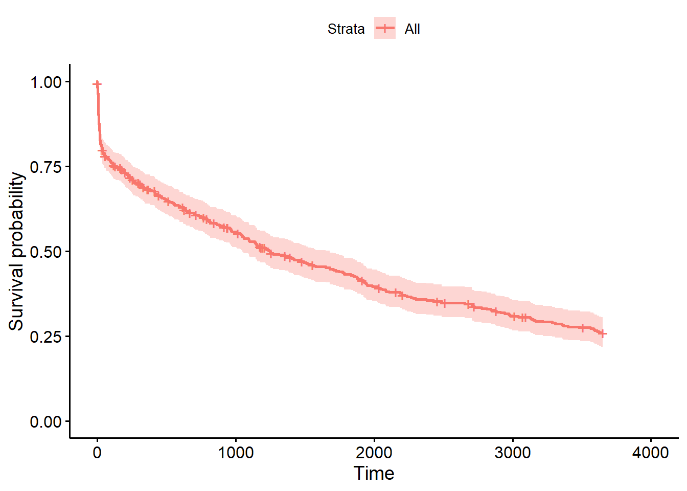
To compute the Kaplan-Meier estimates, we use the function survfit() on s. If we want the overall survival, we write:
And plot the results with:

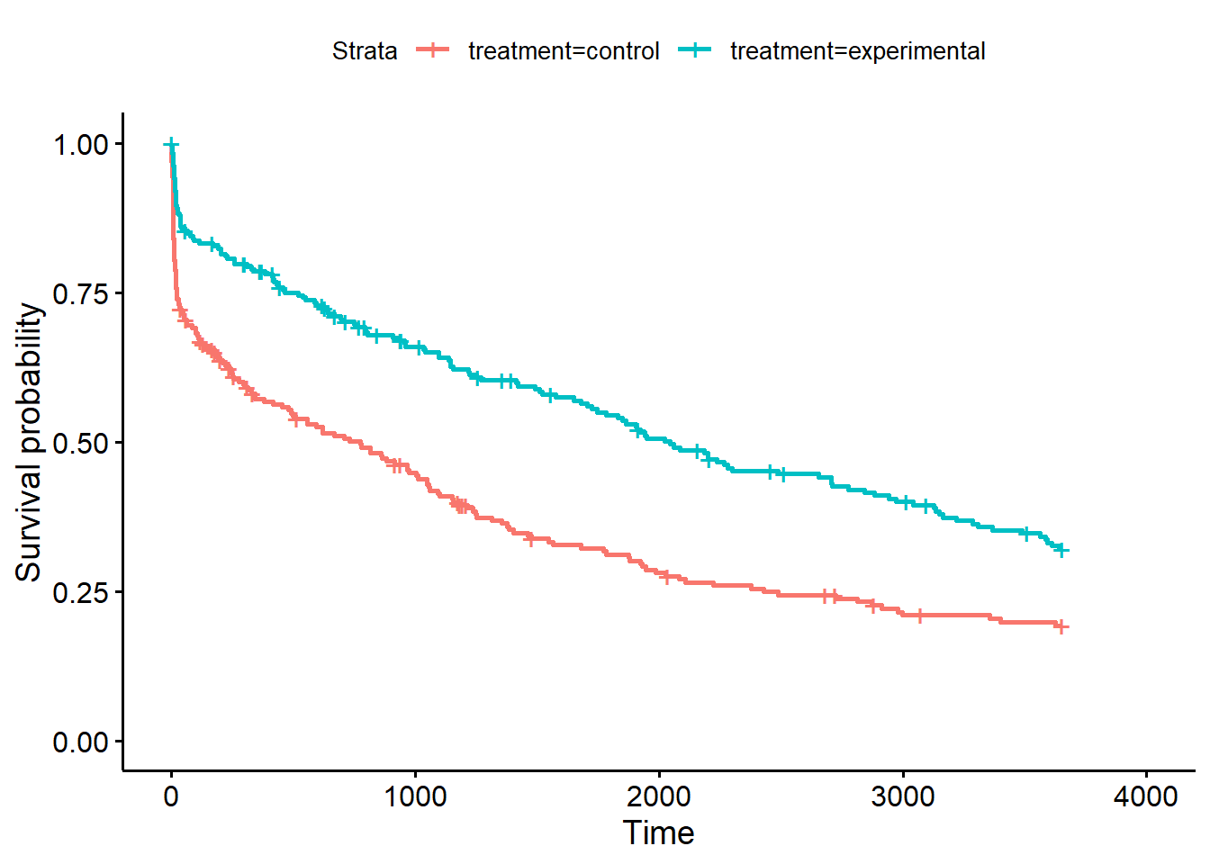
However, it is more interesting to compare the survival of different groups. Lets compare the survival of the experimental treatment group vs. the control group from the variable treatment:

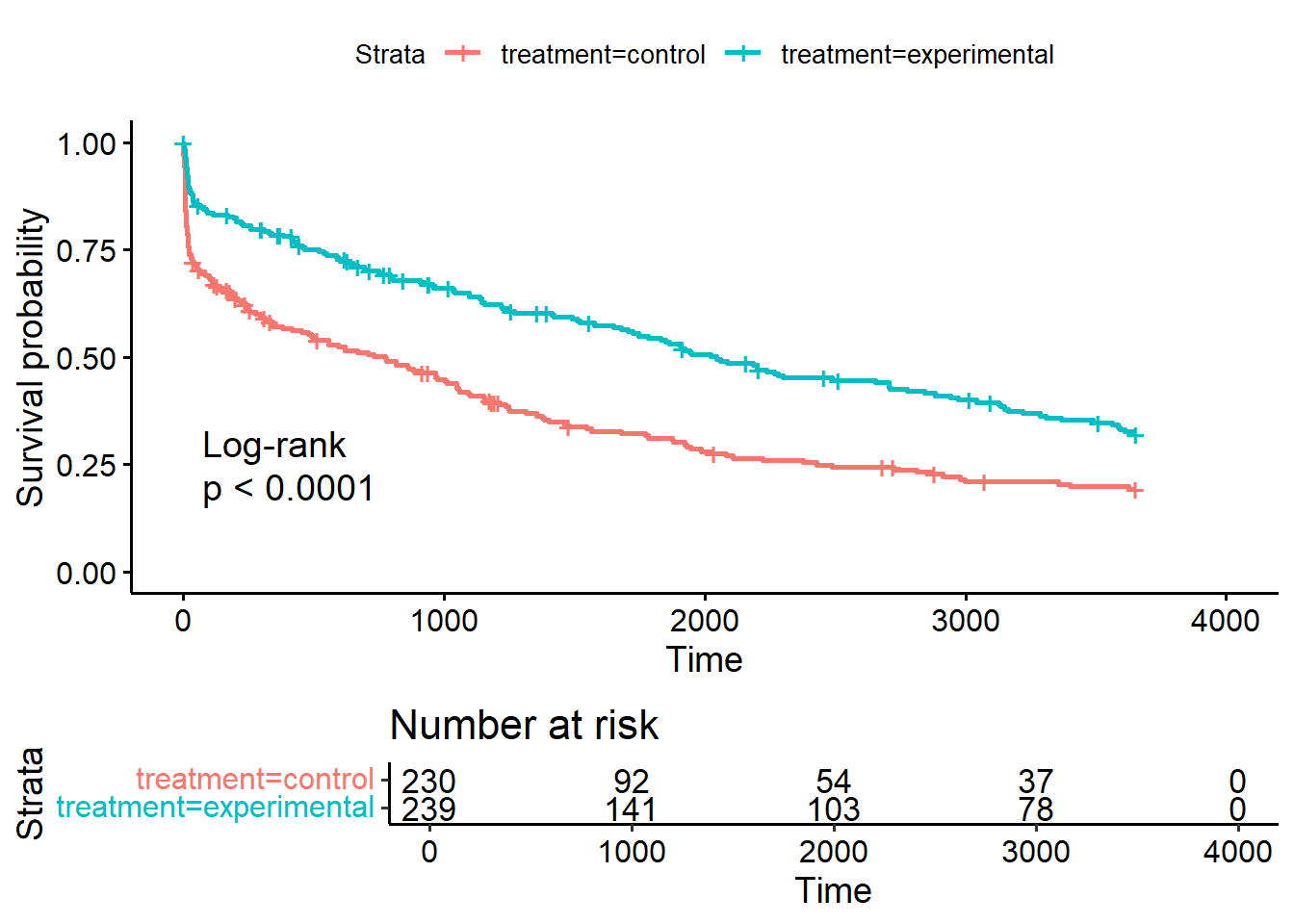
The ggsurvplot() function also has a lot of nice additional options. risk.table=TRUE adds the a table for the number at risk under the plot, pval=TRUE adds the p-value of the log-rank test comparing the survival of the two groups and pval.method=TRUE prints the name of the test above the p-value:

It is also possible to look at the Kaplan-Meier estimates as numbers directly by calling summary(sf_treat), but because the output is rather long, we will not print it here.