Chapter 2 Data exploration
2.1 Functions
Besides the data structures you have learned about in the last chapter, there is another important concept you need to learn about when using R: the function. In principle, you can imagine a function as a little machine that takes some input (usually some kind of data), processes that input in a certain way and gives back the result as output.
There are functions for almost every computation and statistical test you might want to do, there are functions to read and write data, to shape and manipulate it, to produce plots and even to write books (this document is written completely in R)! The function mean() for example takes a numeric vector as input and computes the mean of the numbers in the numeric vector:
[1] 42.1.1 Structure of a function
The information that goes into the function is called an argument, the output is called the result. A function can have an arbitrary number of arguments, which are named to tell them apart. The function log() for example takes two arguments: a numeric vector x with numbers you want to take the logarithm of and a single integer base with respect to which the logarithm should be taken :
[1] 1.000000 1.301030 1.4771212.1.2 How to use a function
To find out how a function is used (i.e. what arguments it takes and what kind of result it returns) you can use R’s help. Just put ? in front of the function name (without brackets after the function name). If you run this code, the help page appears in the lower right window in RStudio.
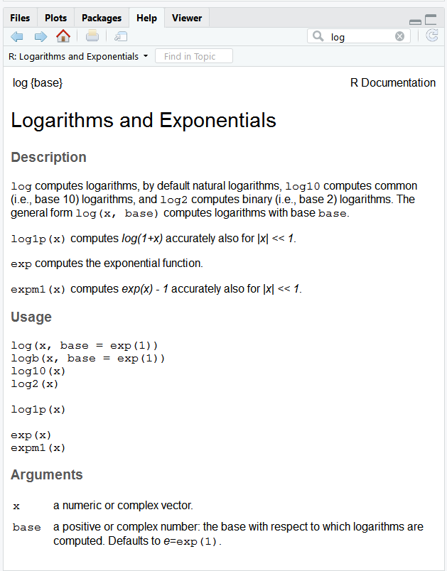
As you can see the help page gives information about a couple of functions, one of which is log(). Besides the description of the arguments you should have a look at the information under Usage. Here you can see that the default value for base is exp(1) (which is approximately 2.72, i.e. Eulers number), whereas there is no default value for x. All arguments that appear solely with their name but without a default value (like x in this case) under Usage are mandatory when you call the function. Not providing these arguments will throw an error. All arguments that have a default value given (like base in this case) can be omitted, in which case R assumes the default value for that argument:
[1] 2.995732 3.401197 3.688879Error in eval(expr, envir, enclos): argument "x" is missing, with no defaultIf you omit the names of the arguments in the function call, R will assume which object belongs to which argument (which may not always be the order you assumed):
[1] 1.000000 1.301030 1.4771212.2 Packages
A basic set of functions are already included in base R, i.e. the software you downloaded when installing R. But since there is a huge community worldwide constantly developing new functions and features for R and since the entirety of all R functions there are is way to big to install at once, most of the functions are bundeled into so called packages. A package is a bundle of functions you can download and install from the Comprehensive R Archive Network (CRAN) (https://cran.r-project.org/). If you visit the site, you can also get an overview over all available packages. You can install a package by using the function install.packages() which takes the package name as a string (i.e. in quotes) as its argument:
If you run this line of code, R goes online and downloads the package lubdridate (Grolemund and Wickham 2011) which contains a number of useful functions for dealing with dates. This operation has to be done only once, so it is one of the rare cases where it makes sense to copy the code directly into the console. If you write it in your script window it is advisable to comment out the code with a # after you have run it once to avoid unnecessarily running it again if you rerun the rest of your script.
Once you have installed the package, its functions are downloaded to your computer but are not accessible yet, because the package has to be activated first. If you try to call a function from a package that is not activated yet (e.g. the function today() from lubridate), you get this error:
Error in today(): could not find function "today"To activate the package, you use the function library(). This function activates the package for your current R session, so you have to do this once per session (a session starts when you open R/Rstudio and ends when you close the window).
[1] "2024-10-02"As you can see the function today()is an example of a function that does not need any argument. Nevertheless you have to call it with brackets () to indicate that you are calling a function rather than a variable called today.
Most packages print some sort of information into the console when they are loaded with library(). Don’t be alarmed by the red color - all of R’s messages, warnings and errors are printed in red. The only messages you should be worried about for this course are the ones starting with Error in:, the rest can be safely ignored for now. However, warning messages can be informative if they appear.
2.3 Loading data into R
Most of the time you will want to use R on your own data so the first thing you will usually do when starting an analysis is to load your data into R. There are generally two ways of loading data into R: either your data is available in an R format such as an .RData file, or your data comes in some non-R format. The former mostly happens when you saved your R workspace for later, the latter will be needed more frequently. For almost every data format there is a dedicated importing function in R. We will start by showing you how to read in non-R formats and then show you how to save and load your R workspace. For demonstration purposes, we have created an example data set simulating a study that compares a novel anti-inflammatory medication to an established medication for sepsis patients. You can find this data in the files example_data.csv and example_data.xlsx.
2.3.1 The working directory
Before we can show you how to import data, you have to get to know another important concept: the working directory. The working directory is basically the folder on your computer where R looks for files to import and where R will create files if you save something. To find out what the current working directory is, use:
R should now print the path to your current woking directory to the console. To change it you can use RStudio. Click Session > Set Working Directory > Choose Directory… in the toolbar in the upper left of your window. You can then navigate to the folder of your choice and click Open.
Now you will see that R prints setwd("<Path to the chosen directory>") to the console. This shows you how you can set your working directory with code: You use the function setwd() and put the correct path in it. Note that R uses / to divide folders, this is different to windows.
Check if it worked by rerunning getwd(). You should now put the data files example_data.csv and example_data.xlsx in the folder you have chosen as your working directory.
2.3.2 Reading data
The comma-separated values (.csv) format is probably the format most widely used in the open-source community. Csv-files can be read into R using the read.csv() function, which expects a csv-file using , as a separator and . as a decimal point. If you happen to have a German file that uses ; and , instead, you have to use read.csv2(). Here, we will however use the standard csv format:
We have not printed the result in this document because it is too long, but if you execute the code yourself you can see that the read.csv() function prints the entire data set (possibly truncated) into the console. If you want to work with the data, it makes sense to store it in a variable:
You can now see the data.frame in the environment window. read.csv() is actually a special case of the more general read_table() function, which can read any kind of text-based tabular data file if you specify the delimiters correctly.
To show you at least one other importing function, we have provided the exact same data set as an excel file. To read this file, you need to install a package with functions for excel files first, for example the package openxlsx (Schauberger and Walker 2023):
If you have another kind of file, just google read R and you file type and you will most likely find an R package for just that.
You should now be able to see example_xlsx and example_csv, two identical data.frames in your working directory. Since they are identical we will work with example_csv from here on.
2.3.3 Saving and loading R data
Sometimes you have worked on some data and want to be able to use your R objects in a later session. In this case, you can save your workspace (the objects listed under Environment) using save() or save.image(). save() takes the names ob the objects you want to save and a name for the file they are saved in. save.image() just saves all of the R objects in your workspace, so you just have to provide the file name:
save(example_csv, file="example.RData") #saves only example_csv
save.image(file="my_workspace.RData") #saves entire workspace
When you now open a new R session and want to pick up where you left, you can load the data with load():
If you want to save a data.frame in some non-R format, almost every read function has a corresponding write function. The most versatile is write.table() which will write a text-file based format, like a tabular separated file or a csv, depending on what you supply in the sep argument.
2.4 Descriptive analysis
Now that we’ve loaded data into R, let’s start with some actual statistics. To get an overview over your data.frame, you can first have a look at it using the View() function. :
The data set contains the following variables:
- patId ID identifying the patient
- gender Gender (‘male’/‘female’)
- treatment Novel anti-inflammatory medication (‘experimental’) vs. established medication (‘control’)
- weight_admission Weight in kg at ICU admission
- weight_discharge Weight in kg at ICU discharge
- age Age in years at ICU admission
- diabetes Does the patient suffer from diabetes? (0 = no, 1 = yes)
- hypertension Does the patient suffer from hypertension (0 = no, 1 = yes)
- apache2_admission Apache II (Acute Physiology and Chronic Health Evaluation II) points at ICU admission, a severity-of-disease classification score (range 0-71)
- apache2_discharge Apache II points at ICU discharge
- qsofa qSOFA (Quick Sequential Organ Failure Assessment) points at ICU admission, a score assessing the risk of sepsis (range 0 to 3)
- crp_admission C-reactive protein in mg/L (an inflammation marker) at ICU admission
- crp_discharge C-reactive protein in mg/L at ICU discharge
- organ_dysfunction_admission Any organ dysfunction at ICU admission (0 = no, 1 = yes)
- organ_dysfunction_discharge Any organ dysfunction at ICU discharge (0 = no, 1 = yes)
- follow_up_time Time until censoring
- follow_up_status Whether the patient died within the follow-up period (0 = no, 1 = yes)
- hospital_death Whether the patient died in the hospital (0 = no, 1 = yes)
- hospital Which hospital the patient was admitted to (A, B or C)
2.4.1 Data types in data.frames
In the lecture you have learned about different data types that variables can have. Here is an overview over the data types R uses to represent these variable types:
| Variable type | R data type | Example variable in example_csv |
|---|---|---|
| Metric | Numeric/Integer | weight_admission, age |
| Ordinal | Integer/Ordered factor | qsofa, apache2_admission |
| Nominal | Unordered factor/Character | gender, treatment |
You are already familiar with the numeric and the character. The integer is a special case of a numeric that only contains whole numbers. The factor on the other hand is a data type that is used to represent categorical variables. It is similar to a character but has only a limited number of values, the so called factor levels. The patient’s name would for example be a character and not a factor because there is a potentially infinite number of values this variable could take. The variable treatment on the other hand can be used as a factor, because the only two values it can take in our data set are experimental and control.
treatment would be an unordered factor, that is, a nominal variable. To represent ordinal variables, you can use the ordered factor that implies an ordering of the factor levels.
You can get an overview over the variable types in the example_csv data.frame by clicking the little blue icon with the triangle next to the example_csv object in the environment window in the upper right corner of RStudio.
When you read the data into R without specifying the data type of every column, R will try to guess them, usually ending up with numeric or integer for all variables containing only numbers and character for variables containing letters or other symbols.
If you want to specify the classes for the read-in process, you can usually pass the argument colClasses with a character vector containing the types for all your variables to the reading function. Because that can be quite a long vector when you have a lot of variables it is often more easy to just let R guess the types and correct them later if necessary.
treatment for example has been read in as a character as you can see using the class() function:
[1] "character"You can turn it into a factor like this:
The factor levels (i.e. the values you newly build factor variable can take) can be extracted with levels():
[1] "control" "experimental"Similarly, one could argue that qsofa should be an ordered factor with
0 < 1 < 2 < 3 , but currently it is represented as numeric.
We can fix that like this:
factor() creates a factor variable from a character vector or existing factor, ordered=TRUE, tells the function to make the factor ordered and the levels= argument specifies the correct order of the levels. With the assignment operator <- we overwrite the old version of qsofa and treatment with the new version. The line breaks are just there so the code is better readable. They don’t change the functionality, just make sure to mark all lines when executing the code.
If you know beforehand that most of the character variables in your data.frame should actually be factors, you can specify this when reading the data in using the argument stringsAsFactors = TRUE:
Have a look at how the description of the data.frame in the environment window changes after running this line of code!
2.4.2 Missing values
When scrolling trough your data, you might have noticed some cells contain NA as a value. NA stands for Not Available and is the value R uses to represent missing values. If you have read in your data from other formats, you might have to check how missing values were coded there and give that information to the read-in function to make sure they are turned in NA.
In most computations you will have to tell R explicitly how to deal with these values (e.g. remove them before computation), else you will get NA as a result. For example, if you want to compute the mean of the variable weight_admission, which contains missing values, you have to set the argument na.rm=TRUE, where na.rm stands for NA remove:
[1] NA[1] 73.560572.4.3 Numerical description
There are functions for many descriptive measures you might want to compute. Most of the time the function name gives a good clue at what the function does. We will go trough the most common ones in the following paragraphs.
Measures of central tendency
Measures of central tendency tell us where the majority of values in the distribution are located. Let’s compute the mean, median and all quartiles of the age variable:
[1] 59.50305[1] 60 0% 25% 50% 75% 100%
19 52 60 67 98 Measures of dispersion
Measures of dispersion describe the spread of the values around a central value. Here you can see how to compute the variance, the standard deviation and the range of a variable. To get the interquartile range just pick the 25- and 75-percentile from the quantile()function above!
[1] 143.6627[1] 11.98594[1] 19 98[1] 19[1] 98Measures of association
Measures of association describe the relationship between two or more variables. In this case there is more than one way to deal with missing values, so instead of the na.rm argument, here we have the argument use= to specify which values to use in case of missing values. For the simple case of looking at correlations between two variables, you can set this argument to use = "complete.obs" which means that only cases without missing values go into the computation. If an observation (i.e. a patient) has NA on at least one of the two variables, this observation is excluded from the computation.
We can compute the Pearson and the Spearman correlation of the age and the admission weight of our patients using the cor() function:
[1] 0.1372897[1] 0.1017086For the association of categorical variables, you will mostly want to look at the frequency tables of the categories. A frequency table for a single variable is produced like this:
     control experimental
         245          255
But you can also use table() to generate cross tables for two variables:
               female male
  control         116  129
  experimental    137  118
General overview
If you want to get an overview over your entire data.frame, the summary() function is convenient. This function can be used for a lot of different kinds of R objects and gives a summary appropriate for whatever the input is. If you give it a data.frame, summary() will give the minimal and maximal value, the 1st and 3rd quartile and the mean and median for every quantitative (i.e. numeric/integer) variable and a frequency table for every factor as well as the number of missing values:
     patId          gender           treatment   weight_admission
 Min.   :  1.0   female:253   control     :245   Min.   :47.00
 1st Qu.:125.8   male  :247   experimental:255   1st Qu.:66.00
 Median :250.5                                   Median :74.00
 Mean   :250.5                                   Mean   :73.56
 3rd Qu.:375.2                                   3rd Qu.:81.00
 Max.   :500.0                                   Max.   :96.00
                                                 NA's   :13
 weight_discharge      age          diabetes       hypertension
 Min.   : 44.00   Min.   :19.0   Min.   :0.0000   Min.   :0.0000
 1st Qu.: 66.00   1st Qu.:52.0   1st Qu.:0.0000   1st Qu.:0.0000
 Median : 73.00   Median :60.0   Median :0.0000   Median :0.0000
 Mean   : 72.79   Mean   :59.5   Mean   :0.1222   Mean   :0.2103
 3rd Qu.: 81.00   3rd Qu.:67.0   3rd Qu.:0.0000   3rd Qu.:0.0000
 Max.   :102.00   Max.   :98.0   Max.   :1.0000   Max.   :1.0000
 NA's   :107      NA's   :9      NA's   :9        NA's   :15
 apache2_admission apache2_discharge     qsofa
 Min.   : 2.00     Min.   : 0.000    Min.   :0.000
 1st Qu.:10.00     1st Qu.: 3.000    1st Qu.:1.000
 Median :13.00     Median : 4.000    Median :1.000
 Mean   :14.09     Mean   : 4.519    Mean   :1.429
 3rd Qu.:17.00     3rd Qu.: 6.000    3rd Qu.:2.000
 Max.   :29.00     Max.   :13.000    Max.   :3.000
 NA's   :12        NA's   :109       NA's   :8
 organ_dysfunction_admission organ_dysfunction_discharge crp_admission
 Min.   :0.0000              Min.   :0.0000              Min.   :  1.00
 1st Qu.:0.0000              1st Qu.:0.0000              1st Qu.: 28.91
 Median :1.0000              Median :0.0000              Median : 60.48
 Mean   :0.6942              Mean   :0.1889              Mean   : 74.16
 3rd Qu.:1.0000              3rd Qu.:0.0000              3rd Qu.:100.72
 Max.   :1.0000              Max.   :1.0000              Max.   :400.00
 NA's   :16                  NA's   :13                  NA's   :7
 crp_discharge    follow_up_time follow_up_status hospital_death   hospital
 Min.   :-58.85   Min.   :   1   Min.   :0.0000   Min.   :0.0000   A:162
 1st Qu.:-57.44   1st Qu.: 110   1st Qu.:0.0000   1st Qu.:0.0000   B:155
 Median :-45.73   Median : 974   Median :1.0000   Median :0.0000   C:183
 Mean   :-24.91   Mean   :1478   Mean   :0.6852   Mean   :0.1976
 3rd Qu.: -9.34   3rd Qu.:2988   3rd Qu.:1.0000   3rd Qu.:0.0000
 Max.   :166.49   Max.   :3650   Max.   :1.0000   Max.   :1.0000
 NA's   :111      NA's   :17     NA's   :14       NA's   :4
2.4.4 Graphical description
For exploration it is also useful to plot the data. R has a number of options for plotting, ranging from simple plots which are quickly made to more elaborate functions and packages that allow you to produce more complex, publication-ready plots with just a little more effort.
For this chapter we will start with the quick and easy ones and go from the most broadly applicable plots that can be used for all types of data to the more exclusive ones that can be used only for data types with a certain scaling.
We will start by introducing the basic plot functions without any customization of labels or axes to give you an overview. When you create plots you want to share, you should of course improve them as, e.g., shown in the last paragraph of the chapter.
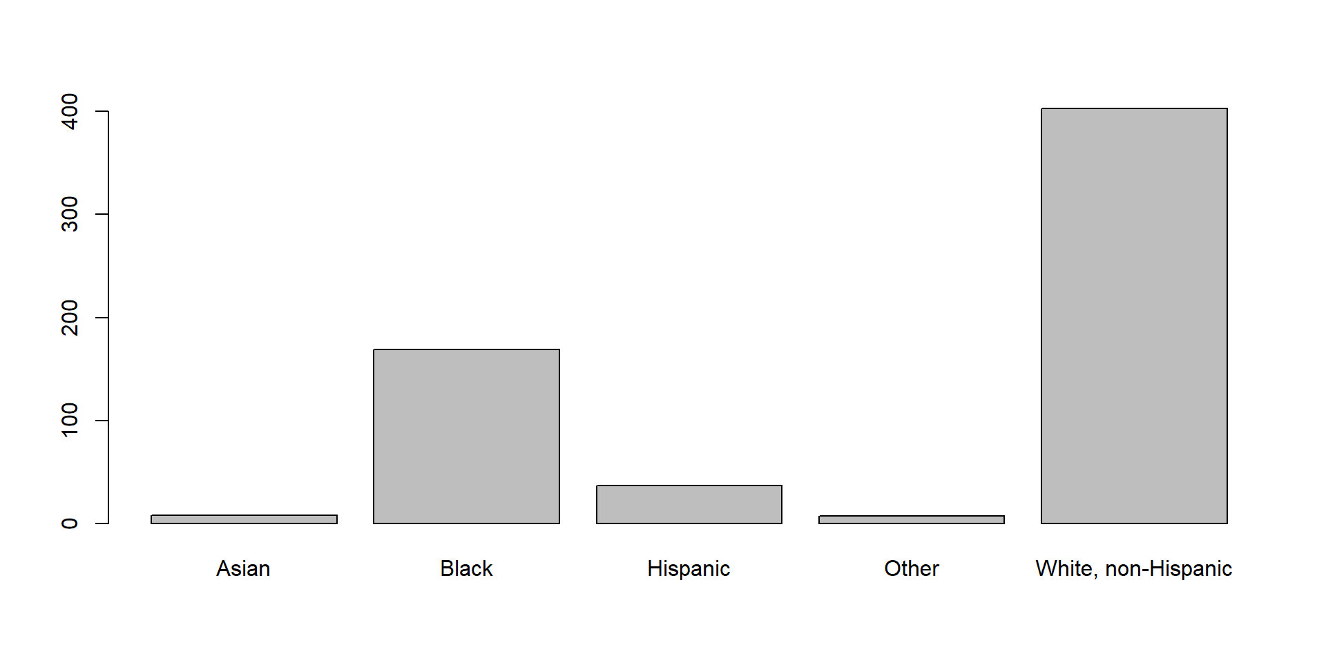
Barplot
A barplot can technically be used on every variable with a finite set of values. The barplot() function takes a frequency table and produces a barplot from it.
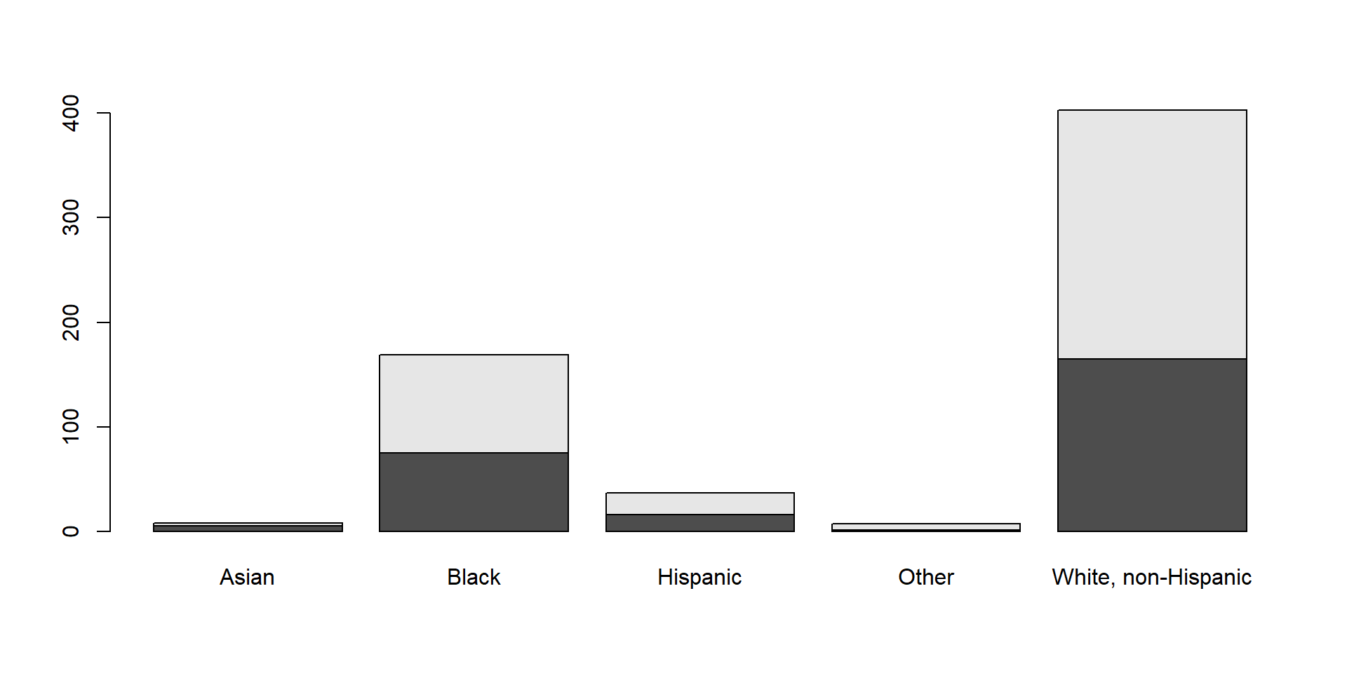
If you give it a crosstable, you get divided barplots:
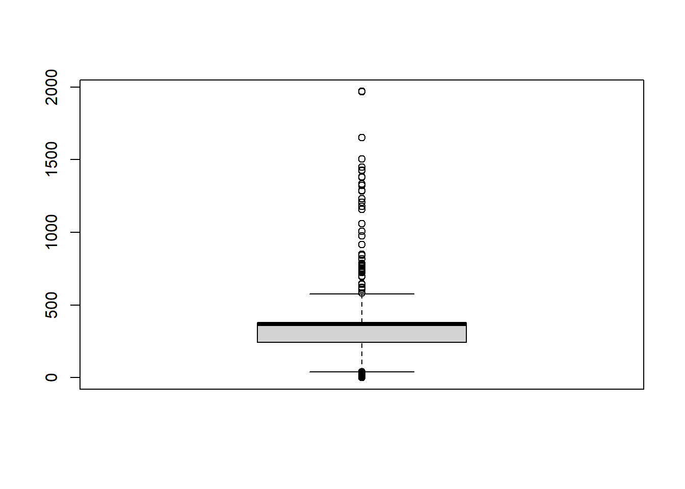
Boxplot
If you have data that is at least ordinal you can use the boxplot() function:
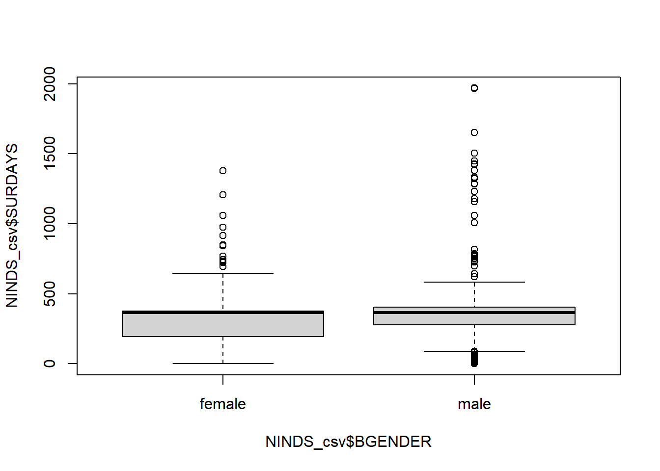
You can also split the boxplot by another (categorical) variable using the ~ sign:
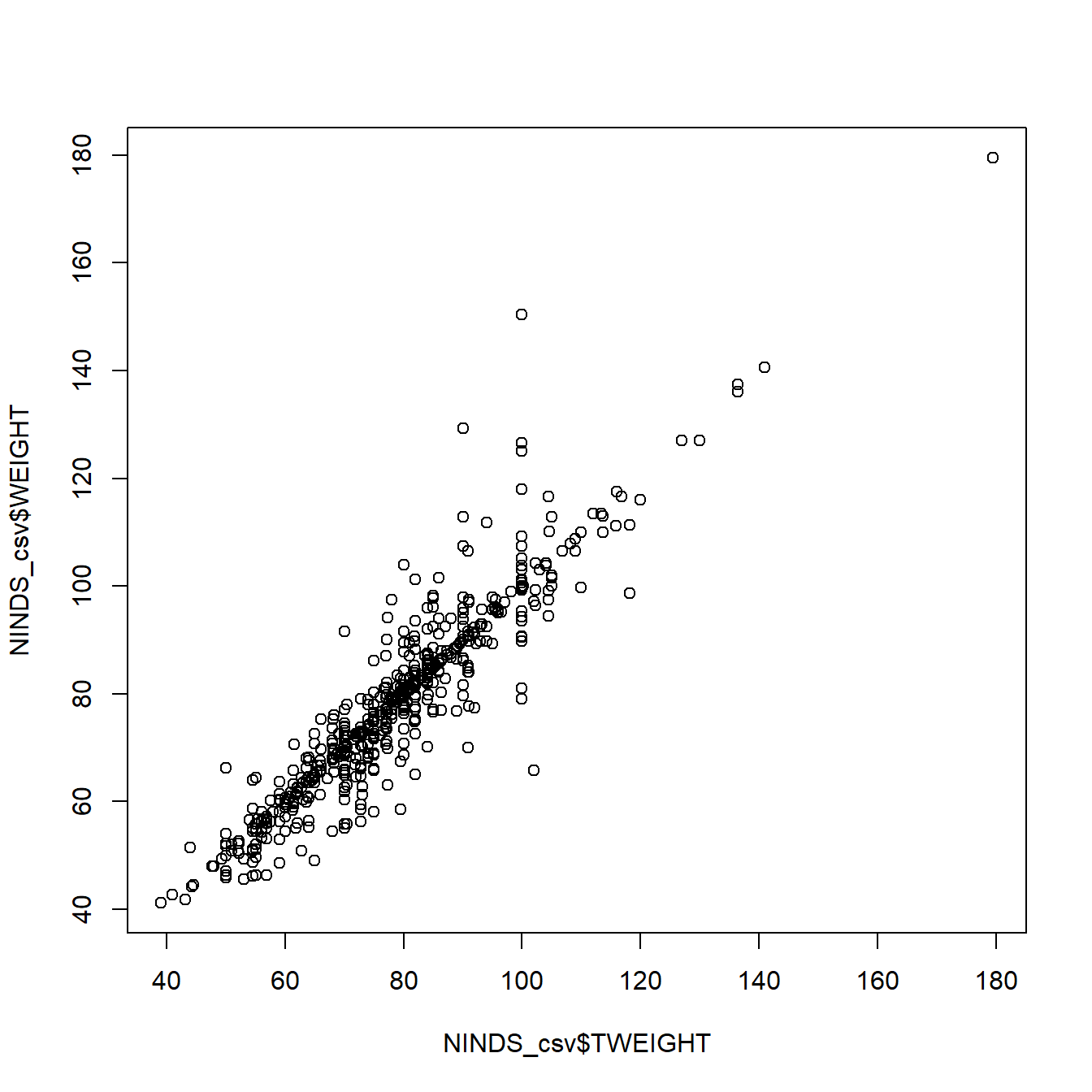
Scatterplot
And we can use scatterplots to get an idea about the relationship of two metric variables:
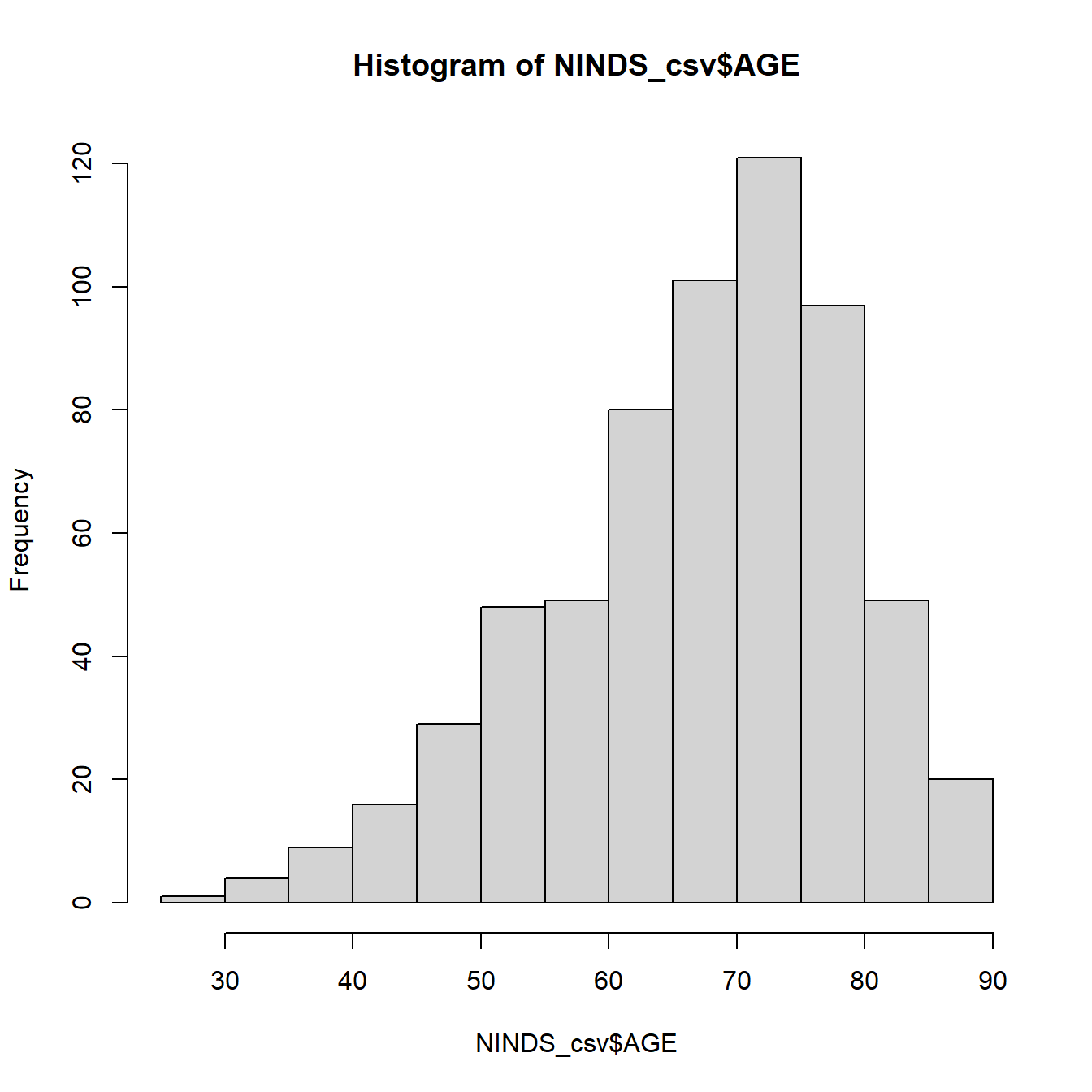
Customisation
Even these basic plots come with a whole lot of customization options. We will exemplary show you a couple of them for the histogram. You can find out about all possible options by going to the help page of the respective function (e.g. ?hist).
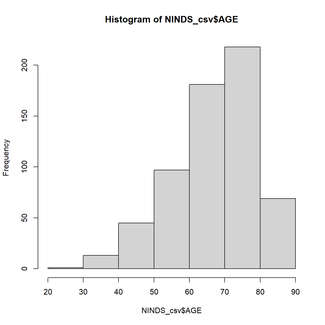
#Add customized x axis and title
hist(example_csv$age, xlab = "Age of subjects in years",
main = "My Title") 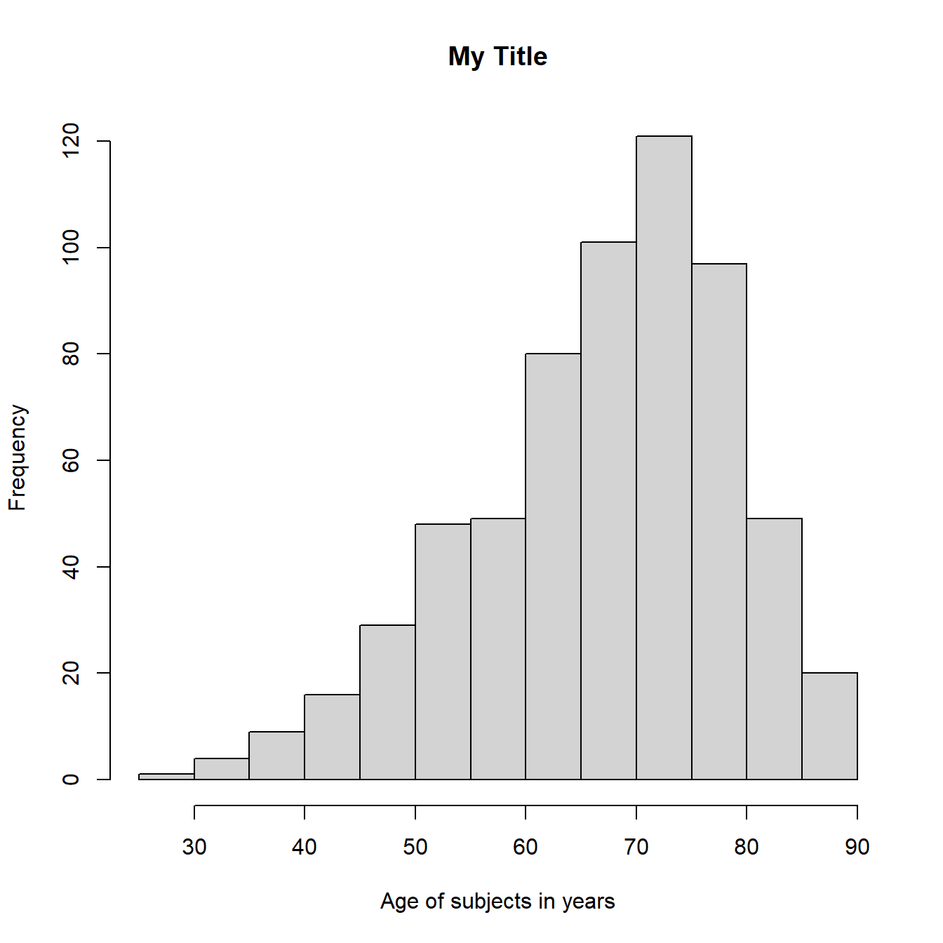
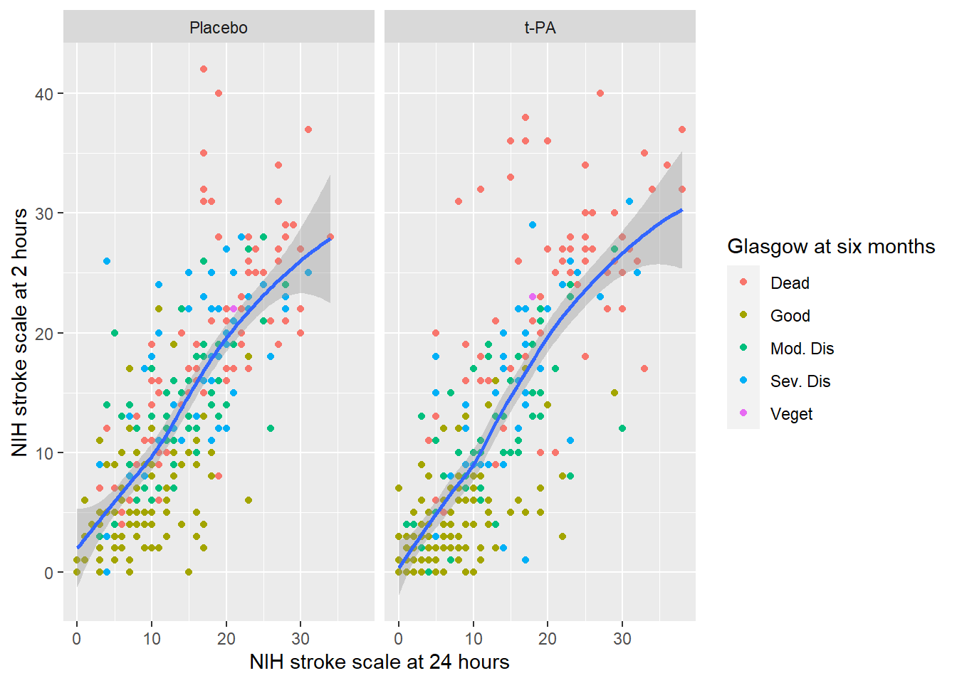
All the plotting functions we have just shown you are useful because they are easy to use. In a later chapter we will introduce the package ggplot2 (Wickham et al. 2024) which allows you to make plots for more complex displays like this one:
2.5 Troubleshooting
Error in file(file, “rt”) : cannot open the connection […] No such file or directory : The file you are trying to open probably does not exist. Check if you spelled the path and file name correctly. Also check if the working directory actually contains the file you are trying to read.
Error in library(“xy”) : there is no package called ‘xy’ : You either misspelled the package name or you have not installed the package yet.
Error in install.packages: object ‘xy’ not found : Have you forgotten to put quotation marks around the package name?
Error in install.packages: package ‘xy’ is not available (for R version x.x.x): Either you misspelled the package name or the package does not exist, or it does not exist for your R version.
Error in plot.new() : figure margins too large : The plot window in the lower right corner of RStudio is too small to display the plot. Make it bigger by dragging the left margin further to the left and rerun the plotting function.