Chapter 5 Advanced Use
In the final chapter we’ll have a look at some of the functionalities of R that make it superior to conventional statistic software. Well have a look at some basic programming you need to write your own functions and show you how to make publication ready plots with ggplot2.
5.1 Programming basics
So far we have used R mainly as a software for statistical analysis, but it is in fact a fully-fledged programming language. Learning the basic structures you need for programming your own functions is actually not very hard, so we’ll show the basic building blocks here.
5.1.1 Defining a function
Apart from using already existing functions in R, you can write you own function if you don’t find one that is doing exactly what you need. For demonstration purposes, let’s define a function mySum() that takes two single numbers firstNumber and secondNumber as input and computes the sum of these numbers:
In this block of code a function is defined and given the name mySum using the assignment operator <-.
The definition of a function always comes in the form function(<arguments>){<body>}. <arguments> is a comma seperated list of the input data you need for you computation and <body> describes the operations that need to be done for the computation. For better readability, we usually enter the <body> over several lines enclosed by {}.
So mySum() expects two input objects firstNumberand secondNumber. In the body, these two are added and the result is assigned the name result. In the next line result is called, to make sure the result gets actually printed when calling the function, then the body closes with }.
After defining the function we can use it:
[1] 7When you execute this line of code, the following happens:
- R looks up the function that is saved under
mySum. - The value 3 is assigned to the internal variable
firstNumberand the value 4 is assigned to the internal variablesecondNumber firstNumber + secondNumberis executed, the result 7 is assigned to the internal variableresultresultis called at the end of the body to make sure its value is returned to the “outside”.- Everything that isn’t explicitly called in the last line of the body stays inside the function. This means neither
resultnorfirstNumberorsecondNumbercan be called outside of the function as the following line shows:
Error in eval(expr, envir, enclos): object 'firstNumber' not found(Translates to Error in eval(expr, envir, enclos): object "firstNumber" not found.)
As you know from the functions you’ve used already, it is also possible to assign default values to some of the arguments. The following function has a default of 10 for secondNumber:
This means if you omit secondNumber in the function call, it is assumed to be 10:
[1] 15But you can overwrite the default:
[1] 7You can also call other functions inside your function. For example you can write a function that computes the mean difference of two vectors:
meandiff <- function(x,y){
    result <- mean(x) - mean(y)
    result
}

v1<-c(1,2,3)
v2<-c(10,20,30)

meandiff(v1,v2)
[1] -185.1.2 Conditional statements
Sometimes you want your code to do one thing in one case and another thing in the other case. For example you could write some code that tests whether a person has fever:
[1] "fever"You can change the value of bodytemp to different values to see how the conditional statement works. In the condition part if(<logical statement>) you test a logical condition of the kind you’ve learned about in the first chapter. Then follows the body {<what to do>} that specifies the code you want to execute if the condition evaluates to TRUE.
In the above code nothing happens if the condition is not met. If you want your code to return a "no fever" for cases where bodytemp < 38, you can extend the statement by an else part:
[1] "no fever"Now, if the condition evaluates to TRUE the block in the first {} is executed, if the condition evaluates to FALSE, the block in the second {} is executed.
Of course you can wrap this in a function to make it easier to use repeatedly:
hasFever <- function(bodytemp){

    if(bodytemp>=38){
        status<-"fever"
    }else{
        status<-"no fever"
    }

    status
}
And try it out with different values:
[1] "no fever"[1] "fever"You can also check different conditions in a row using else if in between. The line breaks are just for readability but make sure you keep track of all the opening and closing brackets!
tempChecker <- function(bodytemp){

    if(bodytemp<36){

        status <- "too cold"

    }else if(bodytemp>=38){

        status <- "too hot"

    }else{

        status <- "normal"
    }

    status
}
Try it out with different numbers:
[1] "too cold"[1] "too hot"[1] "normal"In this code, the conditions are checked in the order they appear in. If the first condition applies, the first block of code is executed, and the rest of the if else statement is ignored. If the first condition is not met, the second condition is evaluated. If it is TRUE the following code block is executed, the rest of the statement is ignored. When the all of the conditions have been tested and evaluated to FALSE, the last code block from the else part is executed.
5.1.3 Loops
The final structure is the loop: A loop allows you to assign repetitive tasks to your computer instead of doing them yourself. The first kind of loop you’ll learn about is the for loop. In this loop you specify the number of repetitions for a task explicitly. The following loop prints the numbers from 1 to 5:
[1] 1
[1] 2
[1] 3
[1] 4
[1] 5
In the () part you define the counting variable, which is often called i (but can have any other name too) and we define the values this counting variable should take (the values 1 to 5 in our case). In the {} part we then define the task for every iteration. print(i) simply tells R to print the value of i into the console. So the above loop has 5 iterations in each of which the current value of i is printed to the console.
Of course we can also have proper computations. For example we can add up alle the numbers from 1 to 1000 with this code:
[1] 500500In the above code the value of result is 0 to begin with. Then the loop enters its first round and the value of result is updated to the current value of result plus the current value of i, so 0 + 1 = 1. Then the second iteration starts and the same happens again: The current value of result is updated by adding the current value of i to it, so result is now 1 + 2 = 3 etc.
Sometimes a repetitive task has to be done until a certain condition is met, but we cannot tell beforehand how many iterations it is going to take. In these cases, we can use the while loop. For example you can count how often you have to add 0.6 until you get to a number that is greater than 1000:
[1] 1667Before the loop starts, both x and counter have the value 0. Then in every iteration, x grows by 0.6 and counter by 1 to count the number of iterations. As soon as the condition in () is not met anylonger (i.e. when x is greater than 1000), the loop stops. As you can see, it takes 1667 iterations to make x greater than 1000.
The previous examples are of course just toy examples to demonstrate the basic functionality of loops. In reality we can use a loop for more practical tasks, for example to create the same kind of graphic for a large number of variables. This brings us to the final chapter of this course: How to produce plots using ggplot2.
5.2 Graphics with ggplot
The package ggplot2 (Wickham et al. 2023) is the most widely used graphics package in R because it gives you control over even the finest details of your graphics while simultaneously doing a lot of the work automatically for you. The syntax takes a bit of getting used to but the results are worth it!
This chapter only touches upon the most commonly used functions of ggplot2. For a comprehensive overview and more useful resources go to https://www.rdocumentation.org/packages/ggplot2/versions/3.4.4.
5.2.1 Structure
In ggplot you build your graphics layer by layer as if you were painting a picture. You start by laying out a blank sheet (with the basic function ggplot()) upon which you add graphical elements (called geoms) and structural elements (like axis labels, colour schemes etc.).
To start, lets install the package and load the NINDS data set again.
Starting with a simple graphic, we want to draw a scatterplot of the NIHSS at 2 hours and 24 hours. In ggplot, we build a graphics object and save it as a variable that is only actually drawn if we call it in the console. We start by laying out a white sheet and call our graphic my_plot:
In this function, we tell the graphic that our data comes from the data set d. But since we haven’t told ggplot what to draw yet, my_plot only produces a blank graph:
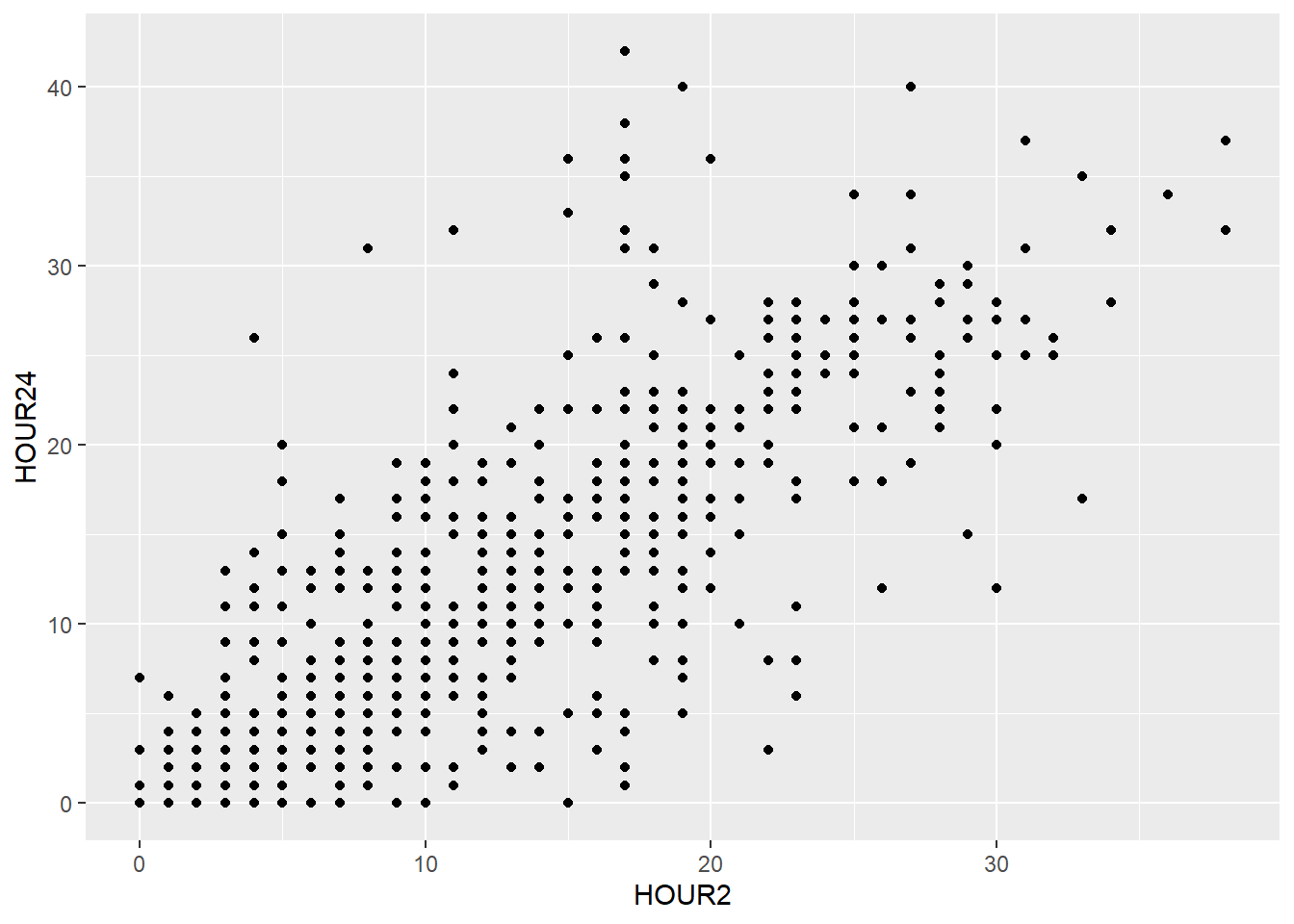
This changes if we add the geom for a scatterplot called geom_point().

The aes() function is part of every geom, it is short for aesthetic and used to specify every feature of the geom that depends on variables from the data frame, like the definition of the x- and y-axis.
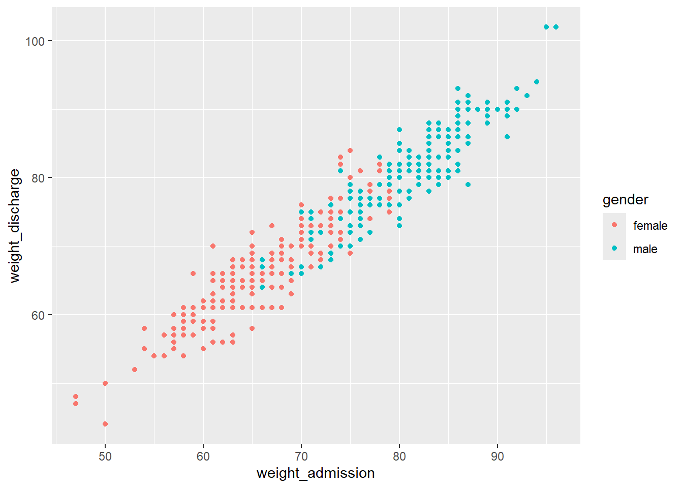
Within aes() we can for example set the color of geom_point() to depend on the gender:
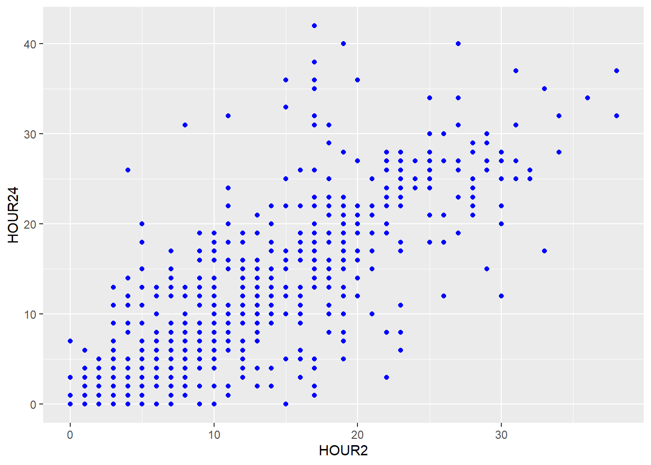
If you want to set a feature of the geom that doesn’t depend on any of the variables (e.g. setting one color for all the points), this is done outside of the aesthetics argument:
You can also add more than one layer to the plot. For example, we could superimpose a (non-linear) regression line by simply adding the geom geom_smooth():
With more than one layer it is easier formatting the code with line breaks. These breaks don’t affect the functionality in any way aside from readability, just make sure you mark all the lines when executing the code. Note, that each line but the last has to end with a + for R to know that those lines belong together.
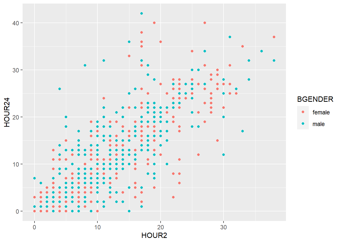
geom_smooth(), too, can be divided with color (e.g. by BGENDER) if we specify it in the color argument of the aesthetics:
my_plot + geom_point(aes(x=HOUR2,y=HOUR24, color=BGENDER)) +
  geom_smooth(aes(x=HOUR2, y=HOUR24, color=BGENDER))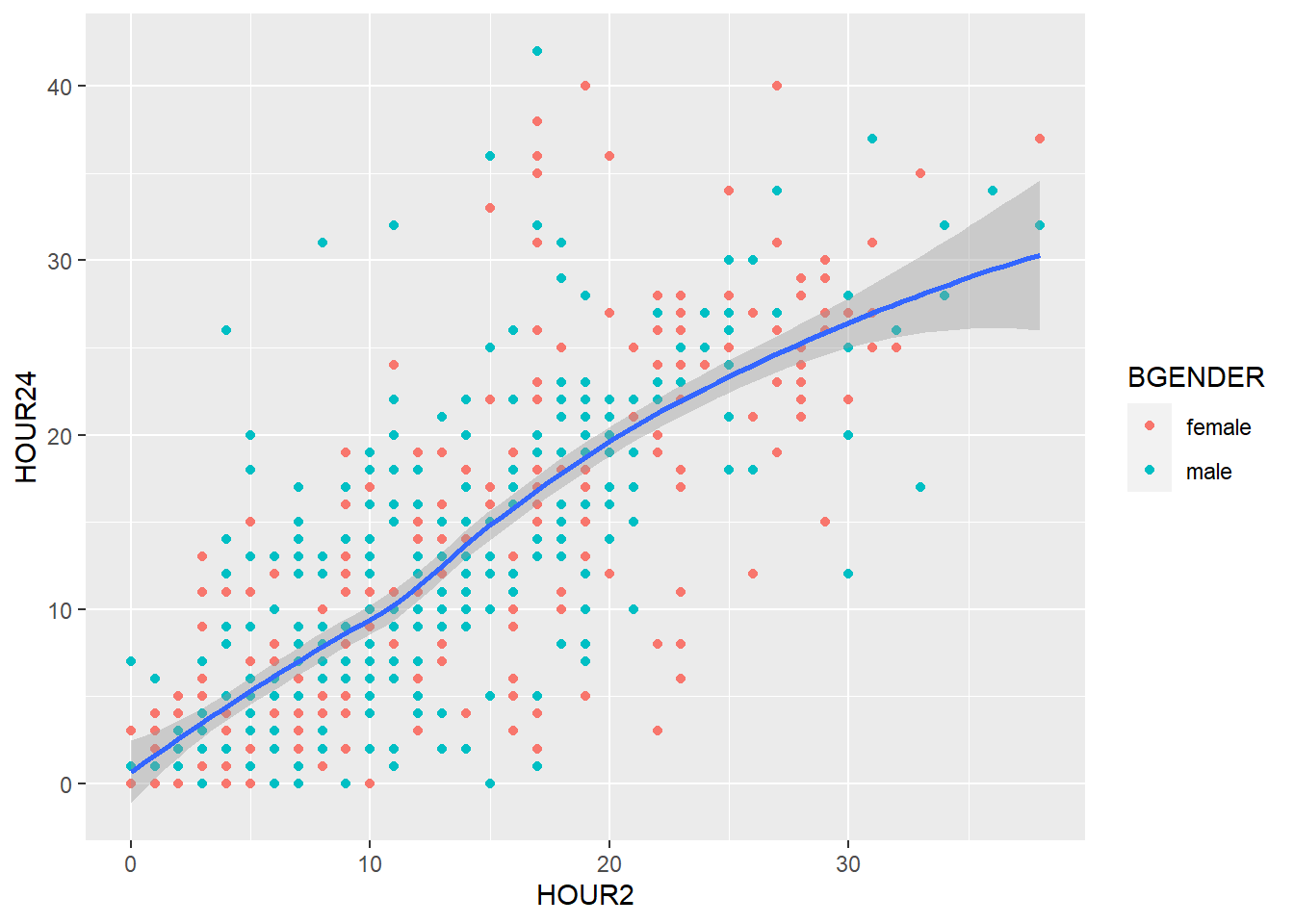
When several layers share the same aesthetics it can be useful to define these aesthetics in the basic plot produced by ggplot():
my_plot2 <- ggplot(data=d, aes(x=HOUR2, y=HOUR24, color=BGENDER))

my_plot2 + geom_point() + geom_smooth()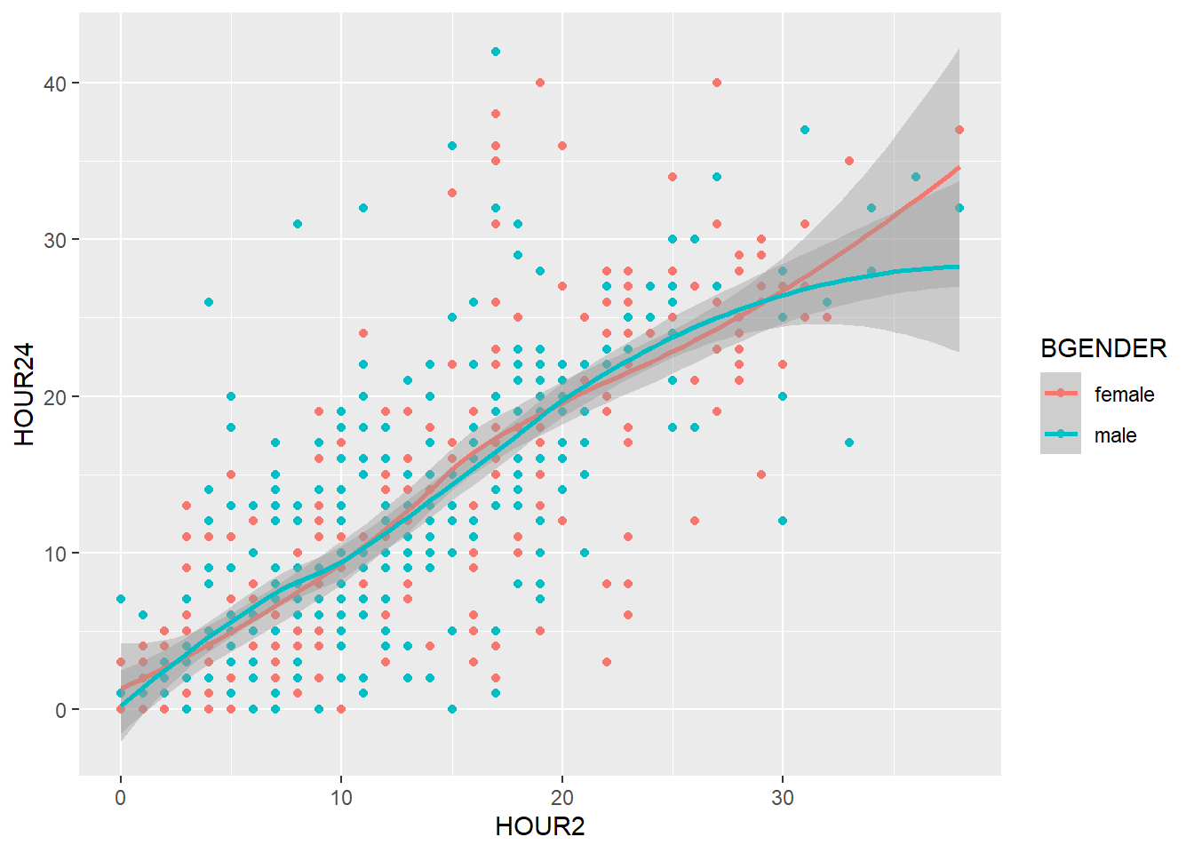
Instead of defining the aesthetics for each geom seperately, geom_point() and geom_smooth() inherit the aesthetics of my_plot2 and the graphic looks exactly the same.
5.2.2 Labels
You can set the labels of your plot using labs().
my_plot2 +
    geom_point() +
    geom_smooth() +
    labs(title = "Scatterplot",
         x= "NIHSS at 2 Hours",
         y="NIHSS at 24 Hours")
5.2.3 Facets
So far we have divided our graph using different colors. It is however also possible to split the graph according to a one or more variables in the data frame using facet_wrap(). To split the graph by presumptive diagnosis (TDX) we write:
my_plot2 +
    geom_point() +
    geom_smooth() +
    labs(title = "Scatterplot",
         x= "NIHSS at 2 Hours",
         y="NIHSS at 24 Hours") +
    facet_wrap(~ TDX)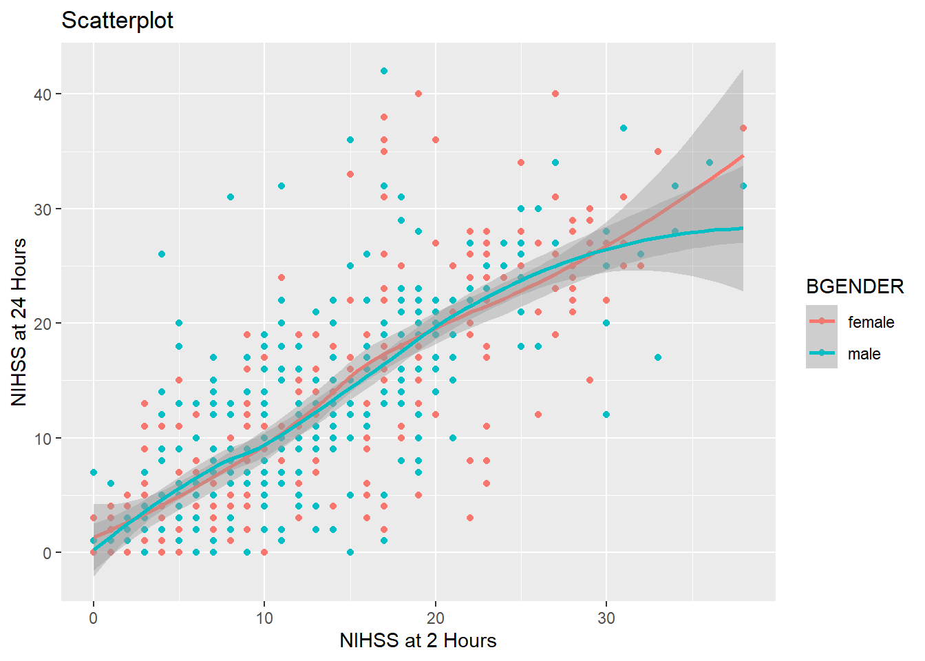
And if we want to split the graph by gender, too, we simply add BGENDER. With ncol=2 we can also tell ggplot to display the plots in two columns:
my_plot2 +
    geom_point() +
    geom_smooth() +
    labs(title = "Scatterplot",
         x= "NIHSS at 2 Hours",
         y="NIHSS at 24 Hours") +
    facet_wrap(~ TDX +  BGENDER, ncol=2)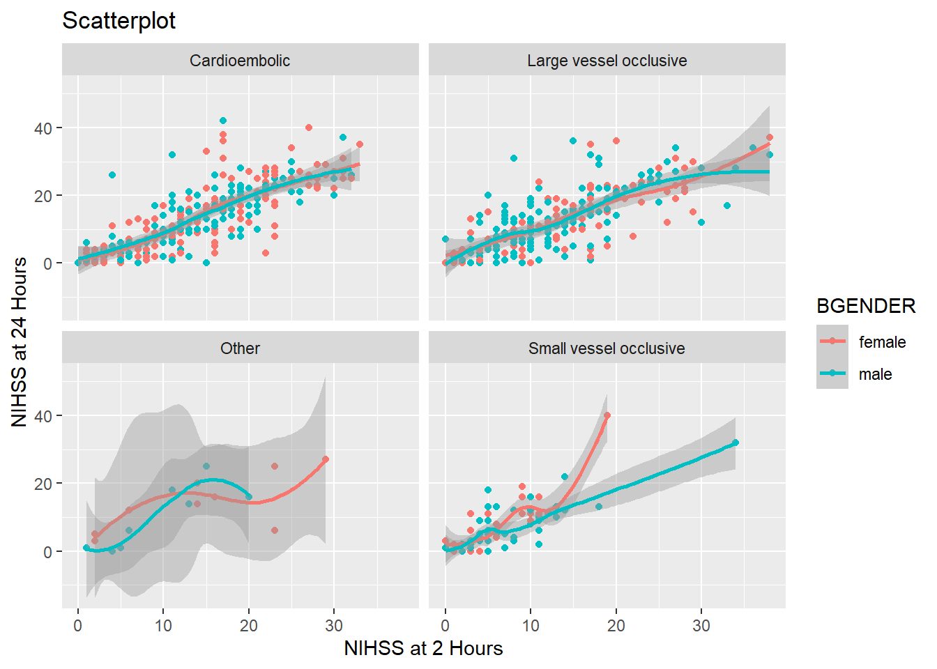
5.2.4 Theme
The theme of a ggplot can be used to change the default appearance of the entire plot or to change specific components of your plot. To find a list of complete themes, go to https://ggplot2.tidyverse.org/reference/ggtheme.html or install the package ggthemes which contains even more complete themes.
The default theme of ggplot is theme_grey, but we can change it like this:
my_plot2 +
    geom_point() +
    geom_smooth() +
    labs(title = "Scatterplot",
         x= "NIHSS at 2 Hours",
         y="NIHSS at 24 Hours") +
    theme_bw()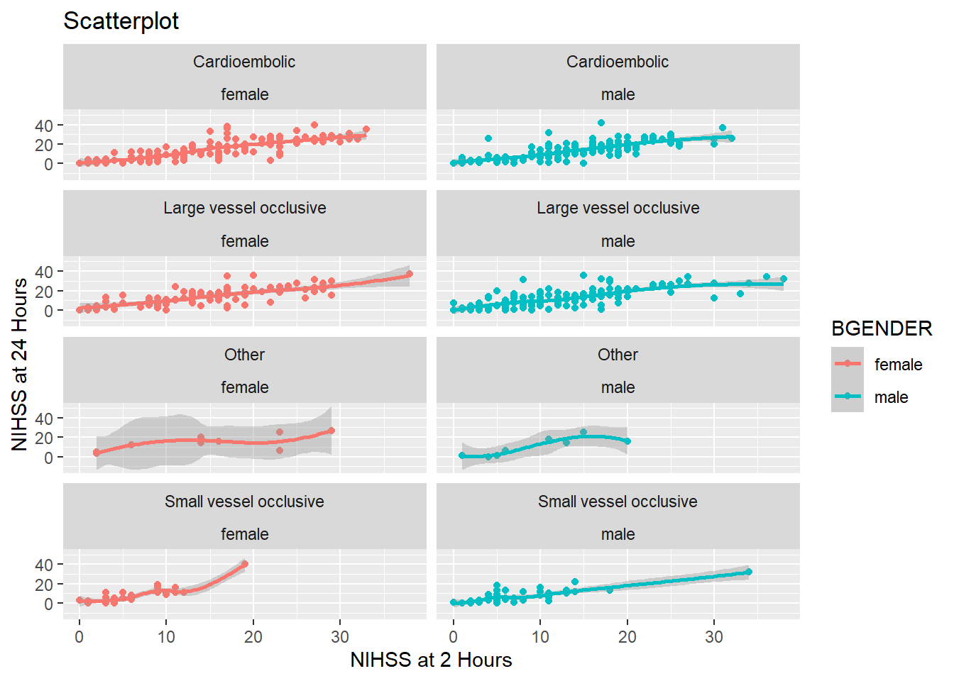
If on the other hand you want to change only certain elements, for example the font size or type of your axis labels, you use theme(), which allows you customize every element of your plot. To change text elements, you give an element_text() to the appropriate argument of theme(). Within element_text you can set the font size, font type, font color, font face and many more aspects. The arguments that take element_text() objects are for example axis.text for the numbers on the axes, axis.title for the axis labels and plot.title for the plot title :
my_plot2 +
    geom_point() +
    geom_smooth() +
    labs(title = "Scatterplot",
         x= "NIHSS at 2 Hours",
         y="NIHSS at 24 Hours") +
    theme(axis.text.x = element_text(size=15),
          axis.text.y= element_text(size=10),
          axis.title = element_text(size=16, face="italic"),
          plot.title = element_text(size=18, face="bold"))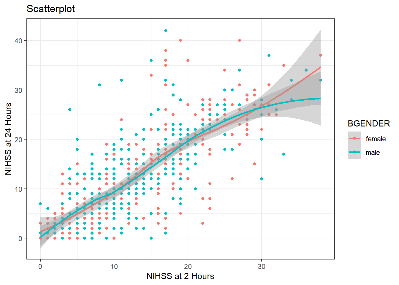
5.3 Further reading
This course aimed at introducing you to the basic ideas of how R works and how it can be of use to you. We have tried to find a balance between keeping it as easy as possible for you to start analysing right away without omitting too much of the underlying concepts. However, we had to leave out a great deal of concepts to fit into these five sessions.
If you are interested in getting to know R better, there is a mountain of useful material. We’ll list a few in the following:
5.3.1 Webpages
- R for Data Science (Wickham, Çetinkaya-Rundel, and Grolemund 2023) available at https://r4ds.hadley.nz/, an online book with very clear and detailed introductions that focuses more on R and how to use it for data analysis and less on traditional statistics.
- Modern Dive (Ismay and Kim 2019) available at https://moderndive.com/, an online book giving an introduction to R but with a strong focus in statistical inference.
- STHDA (http://www.sthda.com/english/wiki/r-basics-quick-and-easy), a website with short, hands-on tutorials explaining how to do a number of statistical analysis including help with output interpretation.
- rdocumentation (https://www.rdocumentation.org/), a collection of the help pages to all the R packages and functions that is a bit more nicely formatted than the help pages whithin R.
5.3.2 Books
- R for Data Science and Modern Dive are also available as physical books
- Discovering Statistics Using R (Field, Miles, and Field 2012), an extensive but very accessible and entertaining introduction to statistics from the very basic to advanced statistical analyses with examples in R