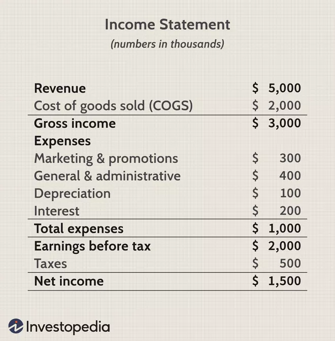
Chapter 4 Financial instruments
4.1 A minimal toolbox, before starting
4.1.1 Compounding / discounting
In this section, the interest rate is assumed to be constant equal to \(r\). Interest rates are almost always expressed per annum in order to be compared properly.
A flow of money is defined by a currency and a date of payment. While it seems obvious that \(1\;USD\neq 1\;EUR\) it is generally less obvious than \(1\;USD\;today\neq1\;USD\;tomorrow\). Think about the promise of principal protected products: is it really an appealing deal ?
Foreign Exchange Rates are the adjustment factor between the value of two unity of currencies. Interest rates are tje adjustment factor between the value of two unity of the same currency paid at different dates. The equalisation of date 1 value with date two value is called Compounding when we move forward in time and discounting when we move backward in time.
Due to the interest paid on deposits, the compounding factor is generally greater than 1 while the discounting factor is generally lower than 1.
Let us now try to give a precise meaning to the above. If \(r=5\%\), what is the value of 1 paid in \(t=2Y\) ? The answer depends on the compounding frequency i.e. the frequency at which the placement is made. The compounding frequency is defined by the number of times \(n\) per year at which the investment is made and re-invested.
If the compounding frequency is equal to \(n =1\), then the value of 1 after 2 years is equal to \(C(t=2,n=1)=(1+r)\times(1+r)\). But if the compounding frequency is equal to 2, then \(C(t=2,n=2)=(1+\frac{r}{2})^4\). More generally:
\[\begin{equation} C(t,n)=(1+\frac{r}{n})^{n\times\frac{t}{n}}. \tag{4.1} \end{equation}\]A way to get rid of the compounding frequency is to agree on an infinite compounding frequency and send \(n\rightarrow\infty\) in formula (4.1) and obtain
\[\begin{equation} C(t)=\underset{n\rightarrow\infty}{lim}C(t,n)=e^{rt}. \tag{4.2} \end{equation}\]Discounting being the inverse operation of compounding, the value, seen from 0, of a flow of 1 at date t is equal to \(B_t=C_t^{-1}.\) The compounding and discounting factors can be interpreted as the exchange rate between two dates.
In the actuarial literature one generally find \(B_t=(1+r_a)^{-t}\) where \(r_a\) stands for the actuarial rate. While the exponential is more clear and allow more tractability, both definition are equivalent indeed with \(r_a=e^r-1.\)
Consider a stream of cash-flows \(X_\tau\) where \(\tau\equiv{t_1,...,t_n}\).
Definition 4.1 (Net Present Value) The Net Present Value of \(X_\tau\) is defined by: \[\begin{align} NPV & =\sum_iB_{t_i}\times X_i \\ & = \sum_i \frac{X_i}{(1+r)^{t_i}} \end{align}\]
When \(X_\tau\) is positive. For a given positive value \(V_0\), the Internal Rate of Return is defined as the value of \(r\) which ensures that: \[V_0=NPV\]
When discounting and compounding one shall remember the two following useful formula. (4.3) is useful for discounting discrete cash flows while formula (4.4) is useful for discounting continuous cash flows.
For \(f<1\):
\[\begin{equation} \sum_{p}^{q}f^{i}=f^{p}\frac{1-f^{q-p}}{1-f} \tag{4.3} \end{equation}\]and:
\[\begin{equation} \int_{0}^{t}e^{-rs}ds=\frac{1}{r}(1-e^{-rt}) \tag{4.4} \end{equation}\]Exercise 4.1 (Perpetuity) The interest rate is supposed constant and equal to \(r\). 1. Compute the NPV of a continuous cash flow paying a continuous coupon \(cds\) from 0 to \(t\). 2. Compute the NPV of a bond paying a discrete yearly coupon \(c\) from 1 to \(n\) plus 1 at date \(n\). 3. Take the limit of both formula to \(+\infty\). Compare and discuss.
4.1.2 Risk measurement
The risk of an asset is that it loses value when one wants to sell it. Markets are such that the average loss and the average gain for one asset are not far from being symmetric.
Financial returns are skewed negatively toward rare important losses. Financial returns also exhibit excess kurtosis as compared to a Gaussian law. Having said that, common P&L are symmetric and the standard deviation (volatility) is a fair first assessment of the risk.
See Asness (2014), Cliff Asness number 1 out 10 peeves: “Volatility” Is for Misguided Geeks; Risk Is Really the Chance of a “Permanent Loss of Capital”.
Having said that daily returns are uncorrelated. As a result, variance formula allow to state that the variance on several days od trading is equal to the sum of variances. In finance then volatility scales as \(\sqrt t\), the square root of time
4.2 Stocks
Readings:
- On Corporate finance: Brealey et al. (2023)
- On equity investing: Graham and Zweig (2003)
- On financial analysis:
4.2.1 Description
Common stock represents equity or an ownership position in a corporation. Payments to common stock are in the form of dividends:
- cash dividend
- stock dividend
- share repurchase
Contrary to payments to bondholders, payments to stockholders are uncertain in both magnitude and timing. Traded in open markets (public vs. private) Important characteristics of common stock:
- Residual claim: stockholders have claim to firm’s cash flows/assets after all obligations to creditors are met
- Limited liability: stockholders may lose their investments, but no more
- Voting rights: stockholders are entitled to vote for the board of directors and on other major decisions
Primary market - underwriting
- Venture capital: A company issues shares to investment partnerships, investment institutions and wealthy individuals.
- Initial public offering (IPO): A company issues shares to general public for the first time (i.e., going public).
Stock issuing to the public is usually organized by investment bank who act as underwriters.
Secondary market (resale market) - Exchanges and OTC
Exchanges: NYSE, AMEX, ECNs OTC: NASDAQ Trading costs: commission, bid-ask spread, price impact Buy on margin Long and short
Warren Buffet: “What’s your favorite stock holding period? Forever!”
The Gordon-Shapiro toy model:
Dividend dynamics : \(D_{t+1}=D_t*(1+g)\)
Price : \[\begin{align*} P &=\sum_{1}^{+\infty}\frac{D(1+g^i)}{(1+r)^i} \\ &= D\times\frac{(1+g)}{r-g} \end{align*}\]
4.3 Rates and bonds
Interest rates are a factor in the valuation of virtually all derivatives. This section introduces a number of different types of interest rate. It introduces fundamental concepts concerned with the way interest rates are measured and analyzed such as IRR and NPV. It explains the compounding frequency used to define an interest rate and the meaning of continuously compounded interest rates, which are used extensively in the analysis of derivatives. It also provides a first presentation of concepts such as forward rates, duration and convexity. Eventually, day count conventions will be introduced.
Volume exchanged across interest rates markets are huge.
4.3.1 Rates
An interest rate is the amount:
- charged on top of the principal by a lender to a borrower,
- earned at a bank or credit union from a deposit account.
There are plenty of interest rates among which:
From Hull (2006).
Treasury rates: Treasury rates are the rates an investor earns on Treasury bills and Treasury bonds. These are the instruments used by a government to borrow in its own currency. It is usually assumed that there is almost no chance that the government of a developed country will default on an obligation denominated in its own currency. A developed country’s Treasury rates are therefore regarded as risk-free.
Overnight Rates: Banks are required to maintain a certain amount of cash, known as a reserve, with the central bank. The reserve requirement for a bank at any time depends on its outstanding assets and liabilities. At the end of a day, some financial institutions typically have surplus funds in their accounts with the central bank while others have requirements for funds. This leads to borrowing and lending overnight. A broker usually matches borrowers and lenders. In the United States, the central bank is the Federal Reserve (often referred to as the Fed) and the overnight rate is called the federal funds rate. The weighted average of the rates in brokered transactions (with weights being determined by the size of the transaction) is termed the effective federal funds rate. This overnight rate is monitored by the Federal Reserve, which may intervene with its own transactions in an attempt to raise or lower it. Other countries have similar systems to the United States. For example, in the United Kingdom, the average of brokered overnight rates is the sterling overnight index average (SONIA); in the eurozone, it is the euro short-term rate (ESTER);1 in Switzerland, it is the Swiss average rate overnight (SARON); in Japan, it is the Tokyo overnight average rate (TONAR).
Repo Rates: Unlike the overnight federal funds rate, repo rates are secured borrowing rates. In a repo (or repurchase agreement), a financial institution that owns securities agrees to sell the securities for a certain price and buy them back at a later time for a slightly higher price. The financial institution is obtaining a loan and the interest it pays is the difference between the price at which the securities are sold and the price at which they are repurchased. The interest rate is referred to as the repo rate. If structured carefully, a repo involves very little credit risk. If the borrower does not honor the agreement, the lending company simply keeps the securities. If the lending company does not keep to its side of the agreement, the original owner of the securities keeps the cash provided by the lending company. The most common type of repo is an overnight repo, where funds are lent overnight. However, longer-term arrangements, known as term repos, are sometimes used. Because it is a secured rate, a repo rate is theoretically very slightly below the corresponding fed funds rate. The secured overnight financing rate (SOFR) is an important volume-weighted median average of the rates on overnight repo transactions in the United States.
For a specific family of rates the yield curve \(r_\tau\) is the set of of rates observed or computed at different maturities from bond prices. Some also refer to the yield curve as \(r_.\) as the value of rates for any possible maturity, extrapolated from the observed yield curve.
Bond rates: the rates implied by a particular bond price
Swap rates: the rates of a particular interbank swap agreement
4.3.2 Mortgages
A fixed-rate mortgage (FRM) is a mortgage loan where the interest rate on the note remains the same through the term of the loan, as opposed to loans where the interest rate may adjust or “float”. As a result, payment amounts and the duration of the loan are fixed and the person who is responsible for paying back the loan benefits from a consistent, single payment and the ability to plan a budget based on this fixed cost.
Exercise 4.2 (mortgage) Do computations
4.3.3 Bullet bond
- Maturity
- Principal
- Coupon
Example. A 3-year bond with principal of $1,000 and annual coupon payment of 5% has the following cash flow:
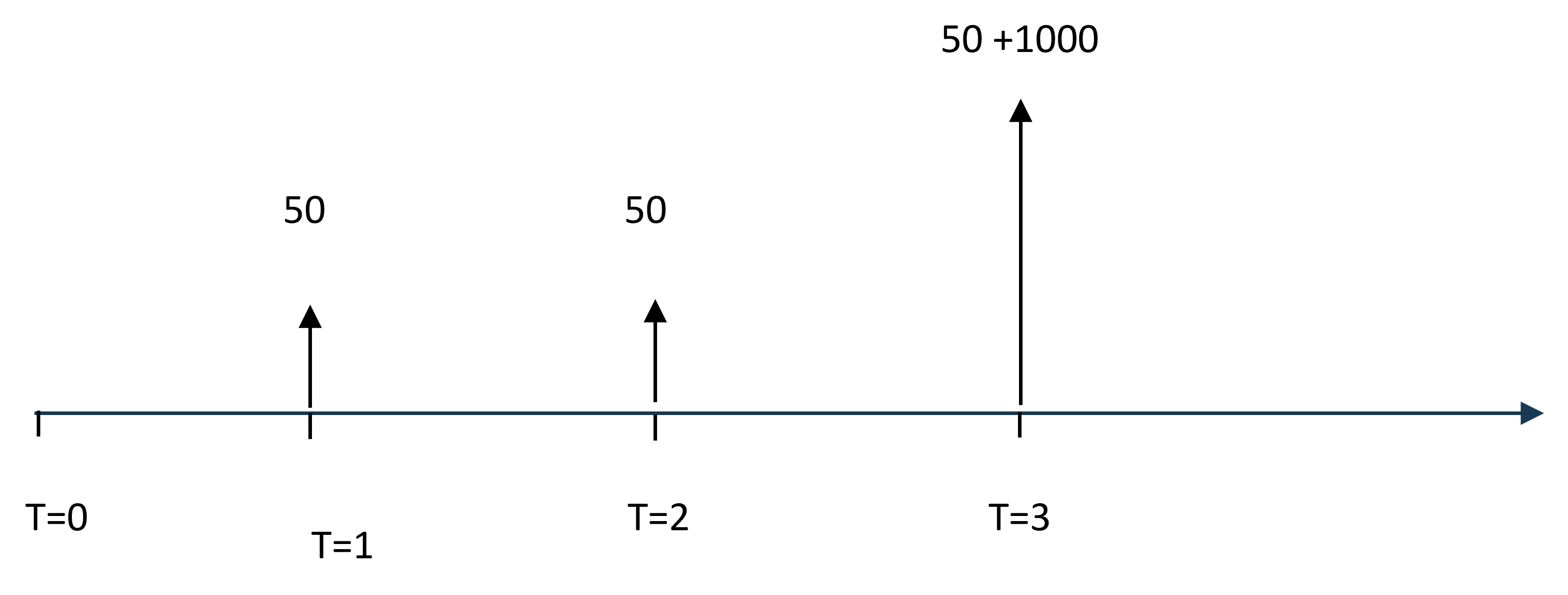
Most market bonds are bullet bonds. The zero-coupon bond is an important particular case of bullet bond.
::: {.definition name = “Zero Coupon Bond” label=“ZC”} A Zero Coupon bond is a bullet bond paying no coupon. Its value is equal to the discount factor. :::
4.3.4 Forward rates
It is possible to fix today the level of a fair interest rate between future dates \(t_1\) and \(t_2\). If you want to borrow money between \(t_1\) and \(t_2\) you can borrow money until \(t_2\) and relend this money until \(t_1\). You should then have: \(\frac{B_{t_2}}{B_{t_1}}=e^{r_{t_1,t_2}\times(t_1,t_2)}.\) As a result
Definition 4.2 (Forward rate) The forward rate between \(t_1\) and \(t_2\) is defined by: \[r_{t_1,t_2}=\frac{t_2\times r_2-t_1\times r_1}{t_2-t_1}\]
The forward rate can also be interpreted as a break-even investment rate. Buy a ZC bond of maturity \(t_2\) and hold it until \(t_1\). At what rate are you better off than having bought directly the \(t_1\) bond instead ?
4.4 Derivatives
A key role in ensuring liquidity as well as disconnecting the needs and utilities of lenders and borrowers.
4.4.1 Forward contracts
4.4.1.1 Definition
A relatively simple derivative is a forward contract. It is an agreement to buy or sell an asset at a certain future time for a certain price. It can be contrasted with a spot contract, which is an agreement to buy or sell an asset almost immediately. A forward contract is traded in the over-the-counter market—usually between two financial institutions or between a financial institution and one of its clients. One of the parties to a forward contract assumes a long position and agrees to buy the underlying asset on a certain specified future date for a certain specified price. The other party assumes a short position and agrees to sell the asset on the same date for the same price. Forward contracts on foreign exchange are very popular. Most large banks employ both spot and forward foreign-exchange traders.
See ??
4.4.1.3 Currency forward
The forward price of a currency at date \(t\) can be obtained spot. Let’s take a EUR/USD example. You are a European corporate who will receive a payment in USD at \(P\) at date \(t\). You are exposed to the variation of the EUR/USD fluctuations. Yearly volatility of that rate is around \(8\%\) so the 6 month volatility is around \(8/\sqrt2\approx5.7\%\).
Interestingly, the FX rate can be fixed today through a Forward Currency Agreement.
If you were to pay the equivalent amount of money in USD, you would be exposed to an increase of the USD. The natural way to match a positive would consist in having an equivalent negative flow at the same date.
Let \(r_€\) and \(r_\$\) the two interest rates prevailing for maturity \(t\) and \(X\) the EUR/USD rate. \(X\) is the amount such that \(1\;EUR=X\;USD\) today. Let us note F the EUR/USD forward rate.
Receiving 1 USD tomorrow can be done in the following manner:
- lend \(B_t^\$\)
- borrow \(XB_t^\$\) in EUR. The 1 USD received tomorrow will have costed you \(\frac{XB_t^\$}{B_t^€}\) in EUR so you are ready to presell it to the equivalent amount:
4.4.1.4 The Quanto effect
In the case of a sure cash-flow, the hedge against FX move can be perfect. But what about hedging an investment into a spider ETF ?
Question: should you hedge your foreign stock investments ?
In case you wish to do so, a natural attempt would be to go for a series of short term forward contracts. For simplicity purpose, take a situation where interest rates in both currencies are equal to zero. The value of the stock, as of today is equal to \(S\) and the EUR/USD is worth \(X\) so that you wealth as of today is equal to \(XS\). You go for a \(\delta\) forward contract So your wealth at date \(\delta\) is equal to
\[ \begin {align} E(P&L) &= E[(S+\delta S)(X+\delta X)]-XS \\ & = E (S \delta X + X \delta S + \delta X \delta S) \\ & = E ( \delta X \delta S) \\ & \underset{\delta\rightarrow0}{\rightarrow} cov(dX,dS) \end {align} \]
Differently stated, the variation of the stock can be hedged by holding the stock the variation of the spot can be hedged by a foward contract but the covariations of the stock and the spot cannot be hedged. The covariance between the spot and the stock very much depends on the realized coorelation. It is bounded in absolute value by the product of the standard deviation which is here approx \(8\%\times15\% = 1.2\%.\)
4.4.2 Futures
Like a forward contract, a futures contract is an agreement between two parties to buy or sell an asset at a certain time in the future for a certain price. Unlike forward contracts, futures contracts are normally traded on an exchange. To make trading possible, the exchange specifies certain standardized features of the contract. As the two parties to the contract do not necessarily know each other, the exchange clearing house stands between them as mentioned earlier. Two large exchanges on which futures contracts are traded are the Chicago Board of Trade (CBOT) and the Chicago Mercantile Exchange (CME), which have now merged to form the CME Group. On these and other exchanges throughout the world, a very wide range of commodities and financial assets form the underlying assets in the various contracts. The commodities include pork bellies, live cattle, sugar, wool, lumber, copper, aluminum, gold, and tin. The financial assets include stock indices, currencies, and Treasury bonds.
4.4.2.1 Commodities futures
Commodities futures are the among the older and larger markets. They allow producers to hedge themselves against variations in commodity prices.
Contango, backwardation and convenience yield are terms used to define the structure of the forward curve. When a market is in contango, the forward price of a futures contract is higher than the spot price. Conversely, when a market is in backwardation, the forward price of the futures contract is lower than the spot price.
Definition 4.3 (Contango) When the spot price is lower than the futures price, the future curve is upward sloping. The market is said to be in contango - the futures contracts are trading at a premium to the spot price. Physically delivered futures contracts may be in a contango because of fundamental factors like storage, financing (cost to carry) and insurance costs. The futures prices can change over time as market participants change their views of the future expected spot price; so the forward curve changes and may move from contango to backwardation.
Definition 4.4 (Backwardation) When the spot price is higher the future curve is downward sloping, or inverted. The market is said to be in backwardation. The futures forward curve may become backwardated in physically-delivered contracts because there may be a benefit to owning the physical material, such as keeping a production process running. This is known as the convenience yield, which is an implied return on warehouse inventory. The convenience yield is inversely related to inventory levels. When warehouse stocks are high, the convenience yield is low and when stocks are low, the yield is high.
Over time, as the futures contract approaches maturity, the futures price will converge with the spot price, otherwise an arbitrage opportunity would exist.
4.4.3 Options
Options are traded both on exchanges and in the over-the-counter market. There are two types of option. A call option gives the holder the right to buy the underlying asset by a certain date for a certain price. A put option gives the holder the right to sell the underlying asset by a certain date for a certain price. The price in the contract is known as the exercise price or strike price; the date in the contract is known as the expiration date or maturity.
American options can be exercised at any time up to the expiration date. European options can be exercised only on the expiration date itself.3 Most of the options that are traded on exchanges are American. In the exchange-traded equity option market, one contract is usually an agreement to buy or sell 100 shares. European options are generally easier to analyze than American options, and some of the properties of an American option are frequently deduced from those of its European counterpart. It should be emphasized that an option gives the holder the right to do something. The holder does not have to exercise this right. This is what distinguishes options from forwards and futures, where the holder is obligated to buy or sell the underlying asset. Whereas it costs nothing to enter into a forward or futures contract, except for margin requirements which will be discussed in Chapter 2, there is a cost to acquiring an option. The largest exchange in the world for trading stock options is the Chicago Board Options Exchange.
Those different pay-offs can be represented in the following manner, as a function of a given underlying:
Present payoffs, combination of payoffs, names intrinsic value, convexity bounds etc.