13 Decision Trees and Random Forests
Decision trees and random forests are powerful non-parametric methods for both classification and regression problems. Them being non-parametric is really useful as you’re not making any assumptions about the functional relationship between your features and targets.
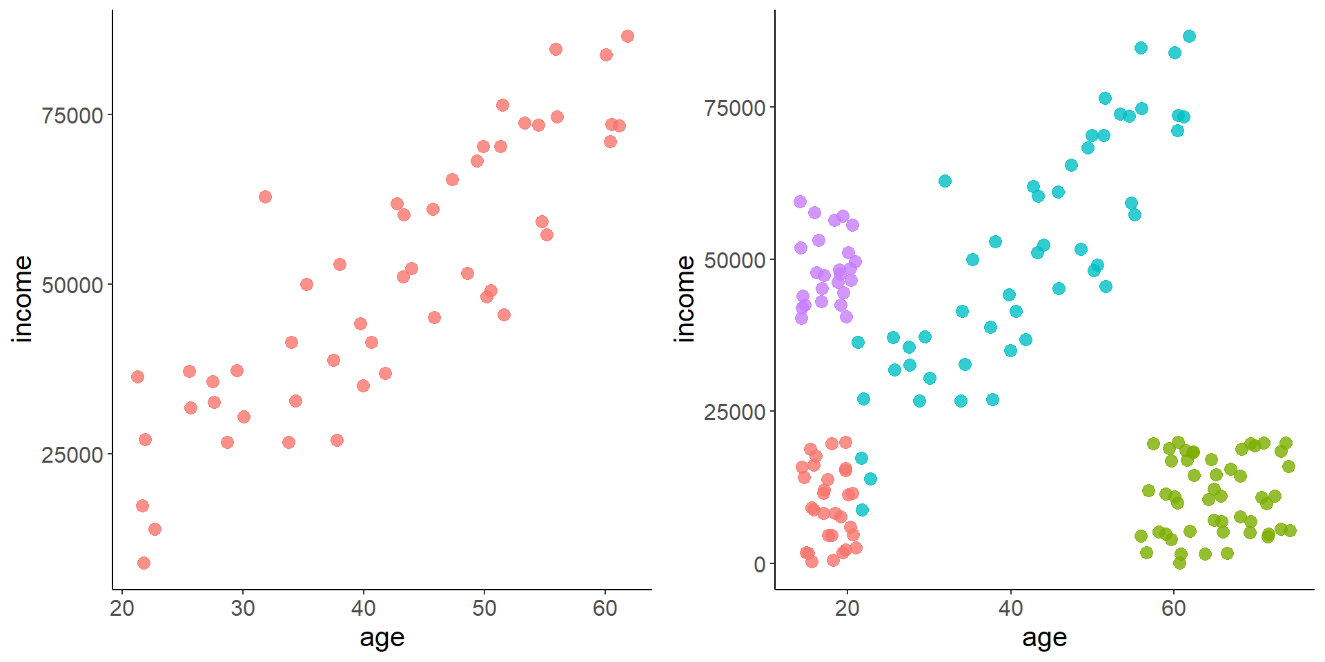
For example, it completely makes sense to fit a linear regression model predicting salary based on age to the figure on the left, but not so much for the figure on the right! There are clearly some very non-linear patterns happening there, so a non-parametric approach might be more fitting.
13.1 Decision Trees
A good way to tackle that graph on the right is through a decision tree. Decision trees are great as they really mirror the way a human makes, well, decisions. It’s essentially a series of if-then splits that divides up the space in a way that most reduces error.
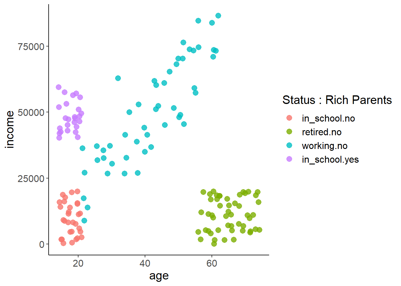
Let’s take a look at the data for that figure on the right. This is data that I simulated, but does a good job of illustrating the logic behind decision trees. We’ll get to real data later! This simulated dataset is looking at how age and working status influences a person’s yearly income. You can see that we have both working status as well as another column for if the person has rich parents (as some students in school do).
income <- read_csv("https://docs.google.com/spreadsheets/d/1ymtFXNEmEc6bOePFgvoHns_x20t16FWJONBuSCieVgY/gviz/tq?tqx=out:csv")
income <- income %>% mutate_if(is.character, as.factor)
summary(income)
## age income group rich_parents
## Min. :14.11 Min. : 88.58 in_school:55 no :130
## 1st Qu.:19.41 1st Qu.:10304.53 retired :50 yes: 25
## Median :40.63 Median :19711.97 working :50
## Mean :40.79 Mean :29461.89
## 3rd Qu.:60.59 3rd Qu.:47705.68
## Max. :74.23 Max. :86588.79Let’s look at the figure again but this time with a legend. Being humans we really naturally start segmenting this up… ‘if you’re in school but don’t have rich parents you make less money than if you have rich parents’ or ‘if you’re retired you don’t make as much money’ or ‘if you’re working you make more money as you age.’ Decision trees use a rather simple algorithm to make these splits for you in a way that best explains the target at hand.
And when you fit and plot a tree to the above data you get this! This makes a lot of sense given the above data. For example, starting at the top if you’re retired or in school you go down the left branch. Then if ‘rich_parents = no’ is true, you go down the left branch again and there you have the predicted income of that branch. But, if ‘rich_parents = no’ was false, or you had rich parents in other words, then your predicted income is much, much higher.

13.1.1 A detour into terminology
We need to take a quick second to talk about the terminology we’ll be using for trees and forests.
Branch - You have left and right branches that take you from one split to another.
Internal node - This refers to each time a feature is divided in two and more splits occur after. The above graph has three internal nodes.
Terminal node - This is now the final groups at the end of each branch. These can also be called leaves.
Pruning - The process of removing terminal nodes
Importance - This refers to how useful a given node is at explaining the target. For regression trees it’s how much a node reduces the \(RSS\). For classification trees it’s how much the Gini index is decreased
Gini Index - The Gini index is a measure of how ‘pure’ a node is. A node is pure is if it contains only one class of your target. So, if a node has all 1’s in it or all zeros in it then it’s pure and suggests that the split that resulted in that node contains a lot of explanatory power. If the node has a mix of 1’s and 0’s, then it’s more impure.
Regression tree - This is a decision tree (or random forest) that is trying to predict a continuous target.
Classification tree - This is a tree/forest that is trying to predict a 0 or 1 class. We won’t do this here, but it operates off identical principles. The only major difference is that instead of using \(RSS\) as it’s error measurement it uses the Gini Index (or some other index if you specify it).
13.1.2 Packages used
Really quick - the book uses the r package tree, but we’re going to use the package rpart. They use almost idential syntax and really only differ by function names. For example, to fit a tree in tree the function is tree(target ~ features) and in rpart it’s rpart(target ~ features). So why use rpart? It makes way better looking graphs!
In order to make those plots you’ll need to install the package rpart.plot.
When we start fitting random forests both the book and here we’ll use the randomForest package.
So, if you haven’t already, go install rpart, rpart.plot, and randomForest.
13.1.3 Decision Tree algorithm
So how do decision trees actually make their decisions as to where to split the data? Well, operate off the same principle as all our other methods - by trying to minimize error in the target. Trees work on both regression and classification problems, and thus try and minimize mean squared error (\(MSE\)) or Gini Index, respectively.
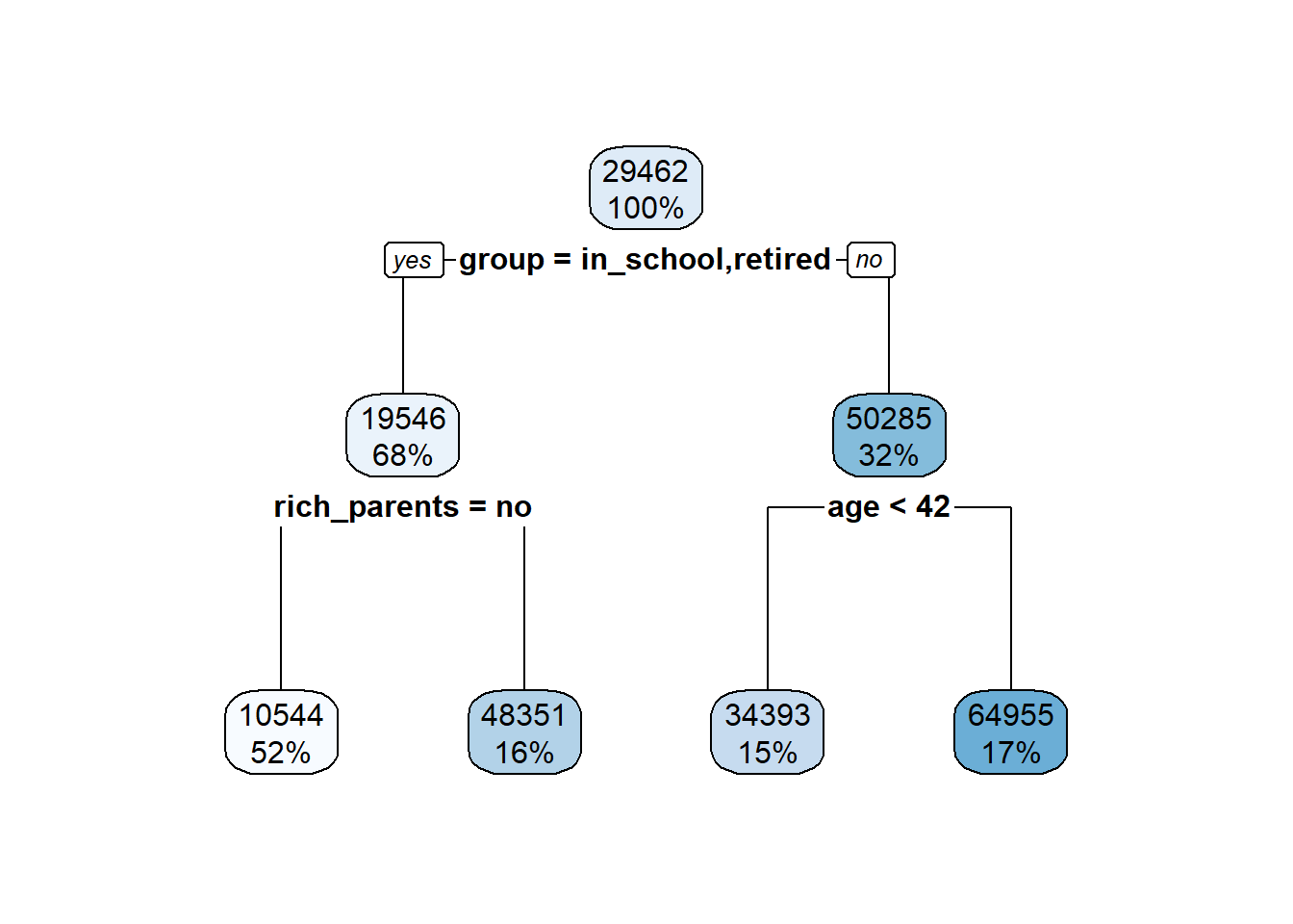
How are the splits (i.e. decisions) for the tree determined? Why is age not first and group not later? It uses something called recursive binary splitting. This starts by considering the whole feature space, and the selects the feature that when split has the largest reduction in error. In the above example it when through and considered each of our three features (age, group, rich_parents) and then what single split within each had the largest reduction in training error. In this case, the largest reduction in error occurred when splitting group into one branch that contained retired and in_school observations, and the other working observations. You now have two regions, and you simply predict that anyone falling into the left branch (in_school or retired) has the mean income value in that region, and anyone falling down the right branch has the mean income value in that region. We can verify this just looking at the mean incomes of each group.
g1 <- income %>% filter(group %in% c('in_school', 'retired'))
mean(g1$income)
## [1] 19545.97g2 <- income %>% filter(group == 'working')
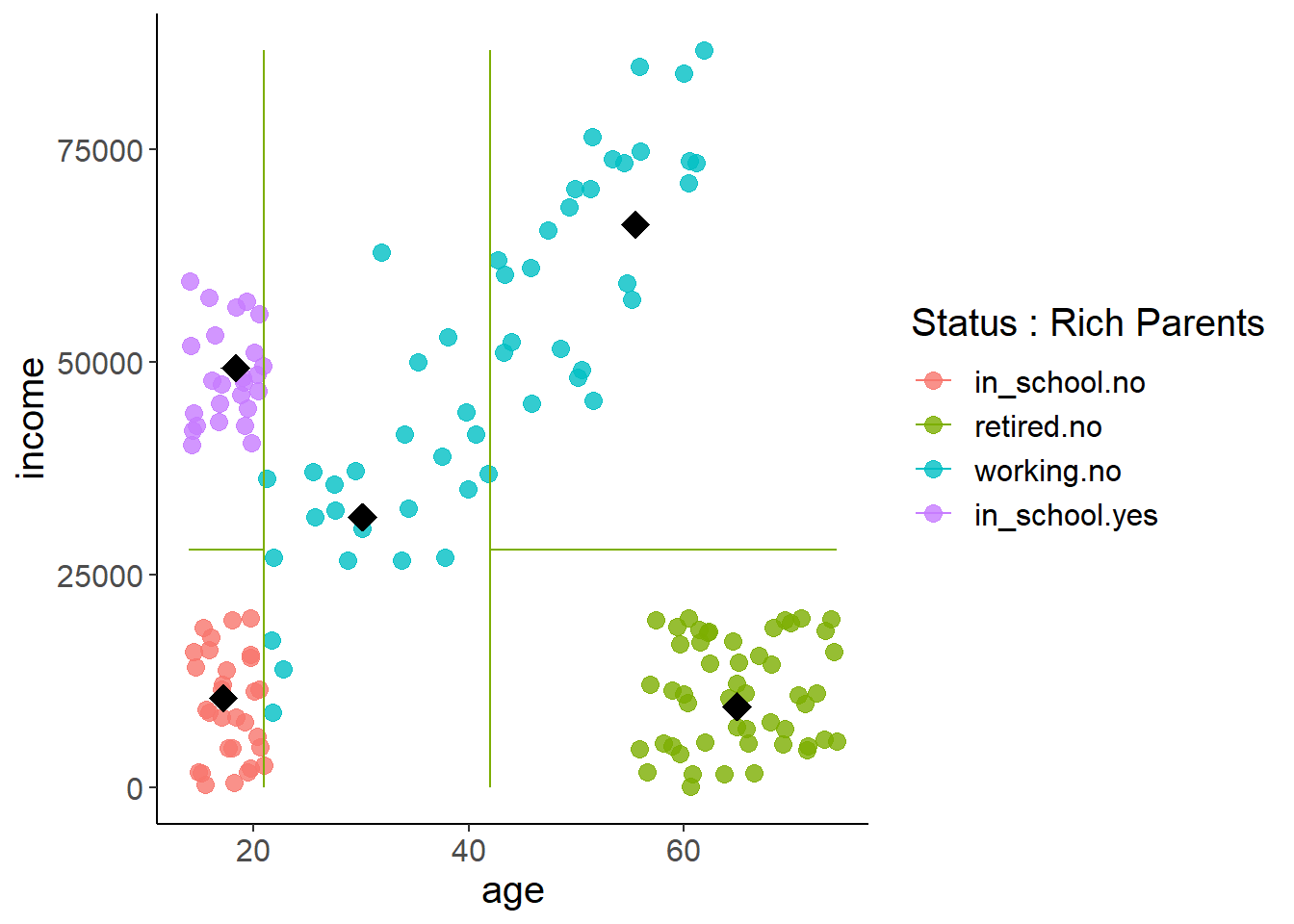
mean(g2$income)## [1] 50285.32With that features divided it’ll go on down a branch and consider another feature, split where the largest reduction in error occurs, then move on. I’ll let you read the book for more details on the specifics of the algorithm. For now, you can see how those mean values at each terminal node maps onto the graph. You can also see with the lines how it draws boundary lines between the segments. Any set of features that falls into that boundary gets a predicted value of the average target, indicated by the black diamond.
The big point I want to illustrate with this intro the general idea of how they operate as well as situations when they can excel. The other point I want to make is that decision trees are just so darn interpretable. This makes them really good for lay audiences. kNN can also tackle this problem, but using that you don’t get any information on the process driving it or relationship between features and target (i.e. you can’t make inference, only predict). And yes, regression approaches can also tackle this with a complex enough model structure (maybe), but have fun showing this table of coefficients to a non-stats-fluent boss!
##                      Estimate Std..Error    t.value     Pr...t..
## (Intercept)       10966.99554  8535.7774  1.2848268 2.008600e-01
## age                 -78.69467   475.1730 -0.1656127 8.686878e-01
## groupretired      -8116.81719 15808.4927 -0.5134466 6.084046e-01
## groupworking     -18848.61690  9377.2365 -2.0100396 4.624407e-02
## rich_parentsyes   38769.44009  2055.6476 18.8599638 3.382040e-41
## age:groupretired    205.90228   517.0400  0.3982328 6.910325e-01
## age:groupworking   1465.25265   483.4253  3.0309805 2.878255e-03
13.1.4 Algorithm Recap
So once again, the basic algorithm is
- Determine which feature when split into two regions (\(R1\) & \(R2\)) results in the greatest reduction in error when predicting the target.
- Assign any observation that falls into \(R1\) the mean of the target values in that region. Any observation that falls into region \(R2\) the mean target value in that region.
Move on to the next feature that allows the next greatest reduction in error.
Repeat until you reach a specified limit for observations in a terminal node (i.e. all terminal nodes must contain > 5 observations).
13.2 Growing our tree to predict AirBnB prices
Let’s now start working with some real data! We’re going to use real AirBnB data to predict rental price based on a bunch of features such as number of bedrooms, bathrooms, host quality, etc. This is the type of model that generates price predictions on any website where you are selling something (e.g. ebay, AirBnB). It takes a bunch of features that you give it and then provides a suggested listing price based off those features.
We’ll start by making a standard decision tree. We’ll see the issues if we let trees grow unchecked, and thus will apply some pruning while also illustrating one of the key problems with decision trees. After that we’ll learn ways around these issues through a technique known as a random forest. Yes, they’ve really gone all-in on the tree terminology.
13.3 Checking out our AirBnB data for this lesson
You all have worked with this data a bit already for your preprocessing lessons. I’ve taken that data and done all the cleaning/imputation/etc. so that it’ll work well with models. Let’s bring in the data and convert everything to factors straight away as they work better with these models. Our target is price and everything else will be a feature.
air <- read_csv("https://docs.google.com/spreadsheets/d/1Lk1v7oXp5B_jK2R84a5PtUAGkdNYQb_Tekl9PkKi7p8/gviz/tq?tqx=out:csv")
air <- air %>% mutate_if(is.character, as.factor)
summary(air)[,2:7] #just looking at a few columns
## cancellation_policy review_scores_rating number_of_reviews
## flexible : 5761 Min. : 20.00 Min. : 0.00
## moderate : 9748 1st Qu.: 95.00 1st Qu.: 2.00
## strict : 783 Median : 97.00 Median : 16.00
## strict_14_with_grace_period:10087 Mean : 95.76 Mean : 45.38
## super_strict_30 : 192 3rd Qu.: 99.00 3rd Qu.: 59.00
## super_strict_60 : 54 Max. :100.00 Max. :963.00
## minimum_nights security_deposit price
## Min. : 1.000 Min. : 0.0 Min. : 0.0
## 1st Qu.: 1.000 1st Qu.: 0.0 1st Qu.: 75.0
## Median : 2.000 Median : 0.0 Median :119.0
## Mean : 7.222 Mean :142.4 Mean :156.5
## 3rd Qu.: 3.000 3rd Qu.:250.0 3rd Qu.:185.0
## Max. :360.000 Max. :999.0 Max. :999.0# air <- sample_n(air, 1000) # Test using a subset if needed!13.3.1 Splitting our data
As always, let’s start by splitting our data into training and test sets. All these random forest models use our common feature ~ target formula structure so we can split out training data into a single data frame that includes both target and features.
split_index <- createDataPartition(air$price, p = 0.8, list = F)

# use index to split data
training <- air[split_index,]
## Warning: The `i` argument of ``[`()` can't be a matrix as of tibble 3.0.0.
## Convert to a vector.
## This warning is displayed once every 8 hours.
## Call `lifecycle::last_warnings()` to see where this warning was generated.features_test <- air[-split_index, !(colnames(air) %in% c('price'))]
target_test <- air[-split_index, 'price']13.3.2 With big trees come big problems
Let’s go ahead and build a single tree with our training data. That trained object contains a lot of information that you can access through the $ operator. For example, let’s look at the variable importance.
air_tree <- rpart(price ~ . ,data = training)
air_tree$variable.importance
## bedrooms accommodates city
## 66335215.9 42525666.4 31599539.7
## room_type bathrooms cancellation_policy
## 31070694.8 29588099.9 19146297.3
## minimum_nights security_deposit property_type
## 17679611.6 16133575.9 16074201.2
## maximum_nights number_of_reviews host_since
## 7196843.6 6997391.2 6531176.6
## reviews_per_month host_response_time review_scores_rating
## 6334936.1 1909018.3 1156157.1
## host_is_superhost bed_type host_identity_verified
## 1068062.2 359049.5 345168.6Plotting this tree is also really easy. Simply call your tree object inside the function rpart.plot().
rpart.plot(air_tree)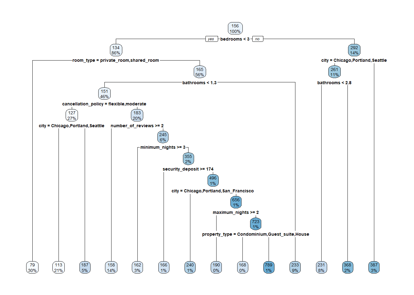
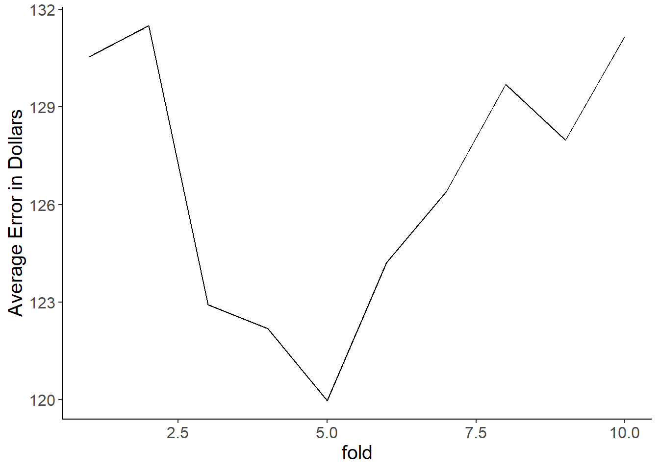
But wow, that’s a lot of branches! This emphasizes problem #1 with decision trees… They will readily overfit if left to their own devices as they will simply keep splitting data until the terminal node threshold is reached. This results in high variance if we predicted price in our test set with this. Let’s look at our test error quick for reference. We do this same as always and see that our decision tree is off on average 105.2 dollars.
tree_preds <- predict(air_tree, newdata = features_test)
tree_mse <- mean((tree_preds - target_test$price)^2)
sqrt(tree_mse)
## [1] 105.203The figure from a quick 10-fold cross-validation shows how much this estimate jumps all over the place.
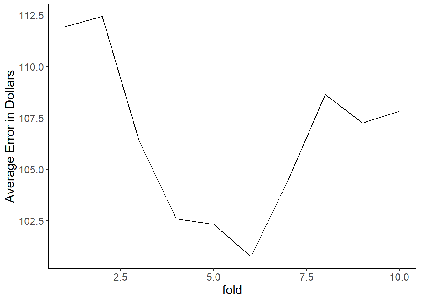
The reason for this brings us to major problem #2. Decision trees are extremely sensitive to small changes in your data. The addition or removal of only one or two points can cause it to build a totally new tree, which in turn affects your ability to stability predict anything. This is even on our large dataset of over 25,000 observations. Here’s a gif image of the 10 trees that were fitted to make the above figure. These differences occur from nothing more than random sampling differences that occurred when making our split_index for cross-validation. Crazy!
13.3.3 Pruning away some leaves
Of course, I wouldn’t show you some apparently awesome method only to demonstrate critical flaws and end the lesson there! We can deal with this in a few ways. The simplest way is by what’s called pruning. Pruning is just what it sounds like - cutting off the terminal nodes (leaves) so that you have fewer decisions in your tree. This makes the model less flexible, which as we should know by now should reduce variance.
We can apply the prune() function to our existing tree. We specific our cost penalty cp = as a way to chop off leaves that don’t improve fit by a certain level (your book has more detail on this). There are additional ways to control pruning. For example. you can use rpart.control() to say what’s the minimum number of observations that need to be in a terminal node.
You could optimize pruning through cross-validation, but we’ll skip that. For now, we’ll just play with the cost complexity to prune it back a bit. You can see that now we have fewer terminal nodes. In other words, the model is using fewer features to fit the data, which should reduce variance.
tree_pruned <- prune(air_tree, cp = 0.045)
rpart.plot(tree_pruned)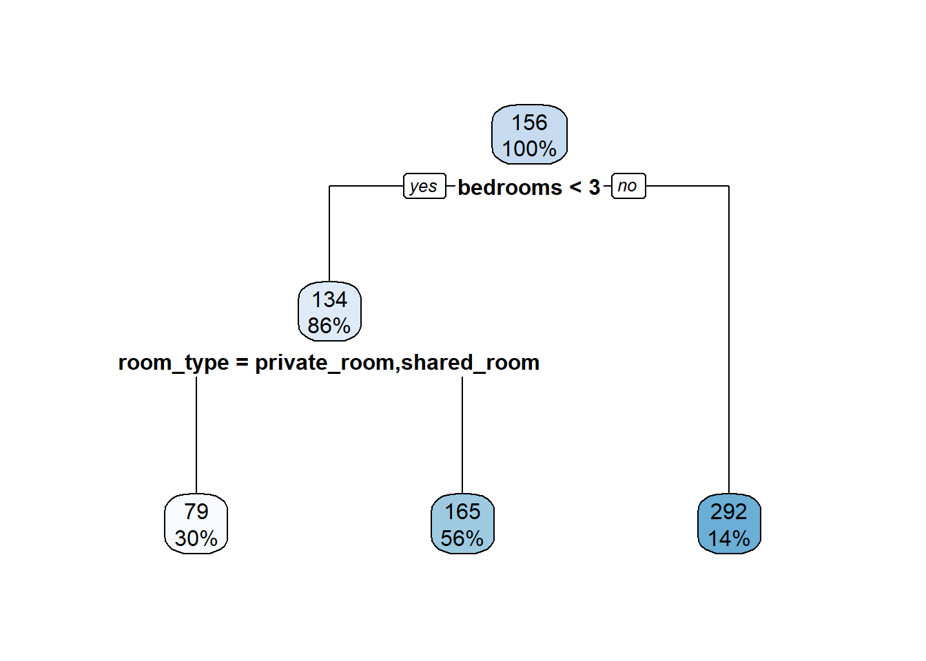
You can see that our error is maybe a bit less variable. The tree will still be highly variable fit-to-fit, but at least it’s not using tons and tons of terminal nodes and overfitting. the con is that in this case the error is actually higher, likely because we pruned too much. Some cross-validation to find the best pruning level would be useful, but it’s still not the best approach so we’ll move on.
13.4 How many trees does it take to make a forest?
As mentioned above, you could cross-validate a range of pruning parameters to maximize the predictive power of your decision tree, or you could take another approach. That other approach is to build lots of trees, each using different subsets of features and then average out those results to make one master predictive model. Making a set of trees and using their predictions creates a random forest.
How random forests work is by generating a large set of trees. The trick is that each tree is generated with a rule governing how many features can be used in a given split. Our AirBnB data had ncol(air) features, and a decision tree can use any one of those features to make the first split, then the rest are available for the 2nd, and so on. Decision trees only use a specified subset determined by the (rule of thumb) formula \(m = p/3\) (or \(m = \sqrt{p}\) for classification trees) where \(m\) is the number of features available for each split and \(p\) is the total number of features in the dataset. The model generates a new set of \(m\) features to choose to split from after each previous split.
A random forest model will make a specified number of trees (say 500) in this manner, and then use all the trees to make a prediction. It makes this prediction by making a prediction for an observation using every single tree, and then taking the average of the predicted responses. So, if for observation \(x_i\) we got predicted target values of 8, 3, 5, 8, and 6 for five trees in the forest. Then the random forest model would predict the target associated with the point \(x_i\) was 6 (sum of responses/number of observations).
This works well because by not allowing all features to be used in the individual tree construction we prevent extremely powerful features from driving the tree generation and allowing other features to have predictive power. This decorrelates the ensemble of trees. This decorrelation helps because although individual models may be off in one direction or another, if you use lots of them their errors should center closer to the true value.
13.4.1 Fitting a forest
Fitting a random forest model is just as simple as fitting a decision tree. We use the package randomForest, which contains the function randomForest(). We specify our formula and training data in the same way as a decision tree. We specify \(m\) using the mtry = argument. This is a regression tree so we’ll use the \(p/3\) formal to determine m. We have 18 features, so we’ll use say m = 6. By default it fits 500 trees, but you can change that using the ntree = argument. Let’s fit our model.
rf_train <- randomForest(price ~ ., data = training, mtry = 6)13.4.2 Estimating feature importance
One problem with random forest models compared to a single decision tree is that we don’t get a nice, handsome graph that clearly shows which features are more important at the top and then works their way down from there. It makes sense that we can’t as each tree in our forest is totally different as it used a different subset of \(m\) predictors for each split, so there’s no intuitive way to visualize that. This is sort of a bummer as one big perk to a decision tree is that they’re so easy to understand.
Although we can’t visualize a tree, we can use the importance() function. The IncNodePurity column indicates how much a given feature reduces the \(RSS\) on average across all the trees in the forest. The bigger the increase in node purity (i.e. the more \(RSS\) was reduced), the more important the feature. So, it’s not a graphical tree, but it is a good way to see which features carry the most explanatory power. Here it makes sense that features such as number of bedrooms in the rental, what city it’s in, and how many people can fit are important for predicting the price.
importance(rf_train)## IncNodePurity
## reviews_per_month 31510397.3
## cancellation_policy 19938006.6
## review_scores_rating 14005935.6
## number_of_reviews 23864032.2
## minimum_nights 21266714.0
## security_deposit 22036408.2
## bed_type 367395.7
## bedrooms 47509542.8
## bathrooms 30919455.6
## accommodates 40957235.0
## room_type 28884541.0
## property_type 15391194.8
## city 36733007.2
## host_identity_verified 8098759.5
## host_is_superhost 4133814.0
## host_response_time 12334380.2
## host_since 26507351.2
## maximum_nights 15291361.913.4.3 Test error of our random forest
Now let’s predict using our random forest model. We can see that our \(mse\) is much lower than the previous methods.
rf_preds <- predict(rf_train, newdata = features_test)
rf_mse <- mean((rf_preds - target_test$price)^2)
sqrt(rf_mse) # boom, wayyy better
## [1] 82.2790213.5 A comparison of methods and applying the model.
Let’s recap here with a quick table comparing our results. We can see that our random forest model far and away dominates the other tree models. Our pruned tree actually did the worst, which is likely because we pruned it too much and it need more flexibility to predict. I also included the prediction from a linear regression model trained as lm(price ~ .). This is a good thing to compare as it suggests that the process of determining price from features is a non-linear one, which is why it did worse.
## [1] 112.7823| model | average error in dollars |
|---|---|
| decision tree w/ 10x CV | 106.46451 |
| pruned tree w/ 10x CV | 126.65859 |
| random forest | 82.27902 |
| linear regression | 112.78232 |
13.6 Wrapping up
Bringing it back to why we created this model in the first place… using this random forest model we can now predict the price of an AirBnB rental within $80 based on a set of 19 features. This is pretty impressive and could for sure be improved with some additional feature engineering and inclusion of a bunch of features that I cut out (the random forest model already takes 10-15 minutes to train!). This type of model could be used in a bunch of ways. Here are two that I can think of.
AirBnB needs to provide a suggested price for people who are listing their rental for a first time. When that renter lists their place they’re going to be entering in their feature values as part of the listing (e.g. bedrooms, bathrooms, location, room type, neighborhood, etc.) as well as other information from their profile that can be turned into features (e.g. do they have other properties, or how long have they been renting on AirBnB). Once all those data are entered they can be kicked into the
predict()of this model and a suggested price and be given.You want to make an app that looks at an AirBnB listing and tells you if it’s a good value or overpriced. That app could scrape all the relevant data off the listing page and kick it into our model. It could then provide a suggested price for that listing. If that listing is well over the suggested price, then it’s overpriced and not a good value. Under the suggested price would indicate it’s a good value and you should go for it.