10 Cross Validation
Last lesson we learned about how it’s critical to split your data into training and test sets, and then validate the quality of model based on how much error between the true targets in the test set and the associated estimated target values. The concept at the heart of this is that we want to make sure we don’t undertrain or overtrain or model which will cause bias and variance (respectively) in the estimates.
This tradeoff can extend to how we choose the size of our training and test sets, and even how many times we create a training and test set. Remember how we used this code to create an index that contained 80% of the values, which we then used to create our split?
ts_split <- createDataPartition(ts$churn, p = 0.8, list = FALSE)How come we didn’t choose p = 0.5 thus splitting half of our data into a training set and the other half into a test set? Why not p = 0.9 and make a tiny test set of only 10% of our data? Too big of a training set (i.e. make p big) can overtrain your model and underestimate test error as you have only a small set of training data to test on. Those data points may by chance miss extreme values that the model would perform poorly on. On the flip side, a small training set would encourage an undertrained model whose performance depends on again what data wound up in that training set!
10.1 Why cross-validation?
You can probably see from the above that the issue is that your model performance can depend not only on the size of a split, but also what data wound up in that split. When you generate your split using createDataPartition() there’s a pseudo random number generator that randomly grabs 80% of the row values (which you use to split). What if that one time you ran it it by chance missed some extreme values which then fell into the test set? What if it by chance captured all the extreme values in the training set? The key idea is that random things happen, and you want to make sure any random event doesn’t give you a biased view of your model performance.
Figure 5.2 does a good job illustrating how our test error can vary wildly if we only use a single split. Each one of those lines represents a single split where the test error (average difference between the true target value and estimated target value) was calculated across a range of models that differed in flexibility (i.e. the number of parameters). They key thing to focus on is that the height on the y-axis (the error) differs greatly each time. This is due just to randomness in the split each time!
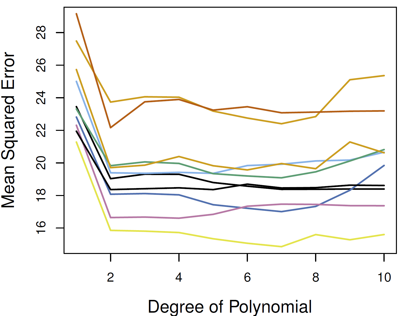
5.2 -right side
How do we get around this? Well, let’s make multiple training sets each with a randomly generated set of index values to split with! This way we can make sure our test error is stable across splits. If it is, it indicates that our split size and model is stable. If our test error jumps all over the place, we need to think about these two things.
10.2 How many splits - from 1 to LOO
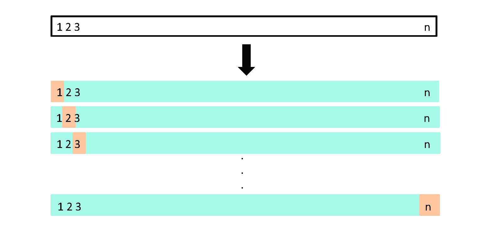
Your book talks about three methods to split your data. One is essentially what we’ve been doing so far where we make a single split and test our model on the training and test set. The other extreme is what’s called Leave-One-Out Cross-Validation or LOOCV. There are two terms there. First, Cross-Validation refers to the process of just splitting your data more than once and validating your model on those various splits (i.e. you validate across splits). The Leave-One-Out is saying that you make the size of your training data set = \(n - 1\) and then your test data set is the single point not in your training data. You calculate the test error with that single point and then go and repeat this process where every single data point will be the test points and all the rest will be the training data. Thus you will split your data \(n\) times and then train/test your model \(n\) times. Your error is then the average error for each time you train/tested!
Figure 5.3 from your book does a great job illustrating how you make multiple fits (each row) where your test set of \(number\:of\: observations - 1\) is the blue area in the row, while the test observation is the tan area. You do this \(n\) times where \(n = number\:of\: observations\)
10.3 k-fold cross-validation
A clear issue with LOOCV is that you have to train a model \(n\) times where \(n = number\:of\: observations\). If you have a million or billion rows of data that would mean training a model a million or billion times. Thus, LOOCV can get out of hand really quick.
A nice balance between the single split method and LOOCV is K-Fold Cross-Validation. \(K\) is simply the number of times (or folds) you split the data and then test the error. A commonly used \(k\) is 5 or 10, and thus you’ll split/train/test your data 5 or 10 times, calculating the error in each split. If your error is stable, you’re good. If not, you need to think more about fit or how big your training/test split is. Overall this balances the computational simplicity of a single train/test split with getting a good idea that your model is estimating error accurately (without going to the extreme of LOOCV).
FYI, cross-validation is considered to be a critical and standard method within industry. Although it seems like a somewhat minor detail, it’s clearly important to assess that your model actually works well. As with preprocessing, it’s these less glamorous details that make the difference between so-so data scientists and good data scientists! Be sure to read the book chapter for the full details!
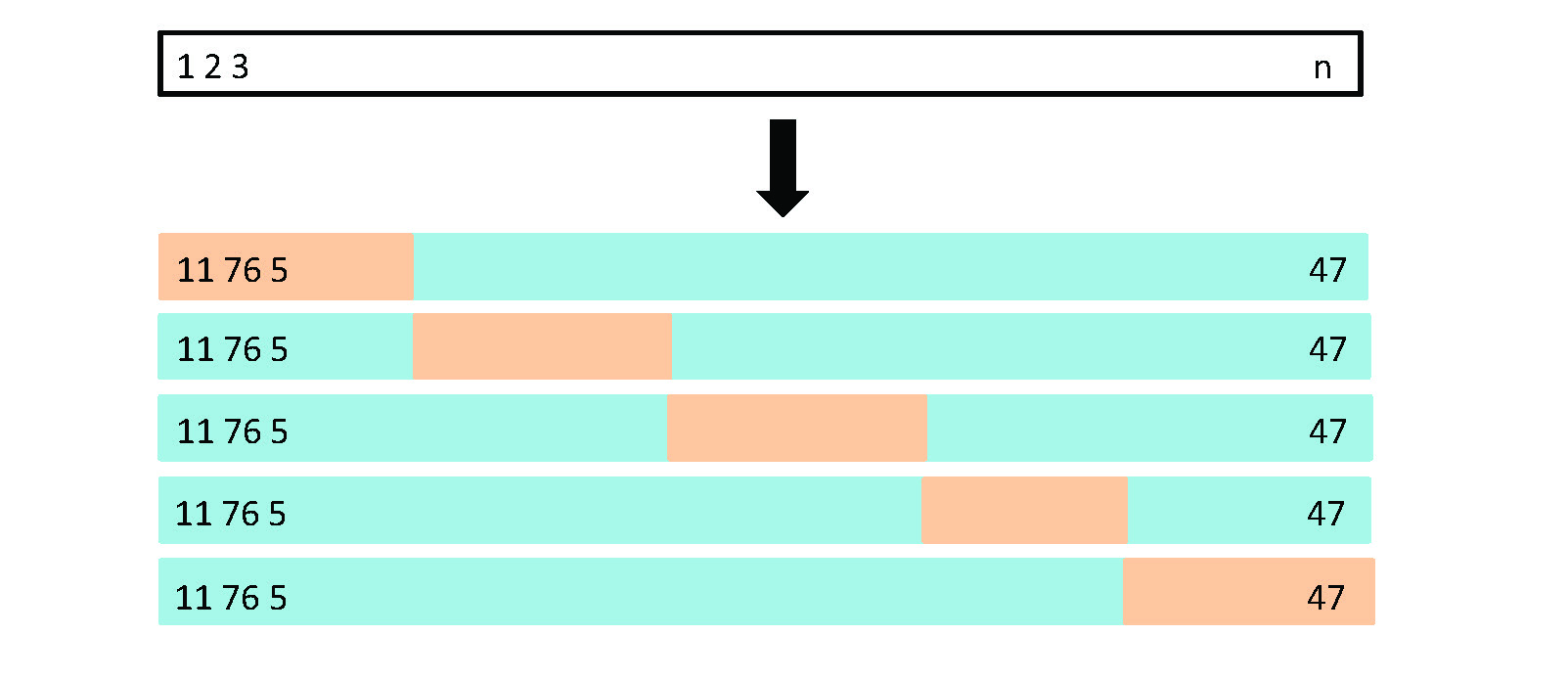
Figure 5.5 from your book illustrates what a 5-fold CV looks like. Note, it’s illustrating someone taking the last 1/5th of the data for the first test fold, then second 1/5th for the 2nd test fold, etc. In reality you take your training and test fold randomly each time. I think they did it that way as it would be messy to illustrate the true way.
10.4 Implementing k-fold CV
Great, we know that k-fold CV is a great way to ensure we fit a quality model. How do we do this? It would be a pain to go and rerun our code 10x times and manually write down the values or store them somewhere. Instead, we’ll use a bit of coding skill to create a bunch of folds, fit our model to each and then look at error across each.
10.4.1 First, our data
Let’s keep working with the telcom data that we used for last week’s example. We’re going to import it and create our dummy variables all in one go.
detach('package:MASS', unload = TRUE)## Warning: 'MASS' namespace cannot be unloaded:
## namespace 'MASS' is imported by 'ipred' so cannot be unloadedlibrary(tidyverse)
# Bring in data
telco <- read_csv("https://docs.google.com/spreadsheets/d/1DZbq89b7IPXXzi_fjmECATtTm4670N_janeqxYLzQv8/gviz/tq?tqx=out:csv")
# Ditch columns we don't need
ts <- telco %>%
select(-ID, -online_security, -online_backup, -tech_support, -streaming_tv, -streaming_movies, -multi_line, -device_protection)
# Create dummy variables
ts_dummy <- dummyVars(churn ~ ., data = ts, fullRank = TRUE)
ts <- predict(ts_dummy, newdata = ts) # apply object
ts <- data.frame(ts) # make a data frame
# go back to original data and get just churn as dummyVars drops it!
churn_vals <- telco %>%
select(churn)
ts <- cbind(ts, churn_vals) # attach it back
ts <- ts %>% # make churn a numeric binary so KNN is happy
mutate(churn = factor(ifelse(ts$churn == 'Yes', 1, 0)))
glimpse(ts) #Always. Check. Your. Data.## Rows: 7,043
## Columns: 17
## $ genderMale <dbl> 0, 1, 1, 1, 0, 0, 1, 0, 0, 1,...
## $ senior <dbl> 0, 0, 0, 0, 0, 0, 0, 0, 0, 0,...
## $ partnerYes <dbl> 1, 0, 0, 0, 0, 0, 0, 0, 1, 0,...
## $ dependentsYes <dbl> 0, 0, 0, 0, 0, 0, 1, 0, 0, 1,...
## $ tenure <dbl> 1, 34, 2, 45, 2, 8, 22, 10, 2...
## $ phoneYes <dbl> 0, 1, 1, 0, 1, 1, 1, 0, 1, 1,...
## $ internetFiber.optic <dbl> 0, 0, 0, 0, 1, 1, 1, 0, 1, 0,...
## $ internetNo <dbl> 0, 0, 0, 0, 0, 0, 0, 0, 0, 0,...
## $ contractOne.year <dbl> 0, 1, 0, 1, 0, 0, 0, 0, 0, 1,...
## $ contractTwo.year <dbl> 0, 0, 0, 0, 0, 0, 0, 0, 0, 0,...
## $ paperless_billYes <dbl> 1, 0, 1, 0, 1, 1, 1, 0, 1, 0,...
## $ payment_methodCredit.card..automatic. <dbl> 0, 0, 0, 0, 0, 0, 1, 0, 0, 0,...
## $ payment_methodElectronic.check <dbl> 1, 0, 0, 0, 1, 1, 0, 0, 1, 0,...
## $ payment_methodMailed.check <dbl> 0, 1, 1, 0, 0, 0, 0, 1, 0, 0,...
## $ monthly_charges <dbl> 29.85, 56.95, 53.85, 42.30, 7...
## $ total_charges <dbl> 29.85, 1889.50, 108.15, 1840....
## $ churn <fct> 0, 0, 1, 0, 1, 1, 0, 0, 1, 0,...10.4.2 Creating your folds
Originally we used createDataPartition() to make our index that we used to split. For example:
split_index <- createDataPartition(ts$churn, p = 0.8, list = FALSE)
head(split_index, 10)
## Resample1
## [1,] 1
## [2,] 2
## [3,] 3
## [4,] 4
## [5,] 5
## [6,] 6
## [7,] 7
## [8,] 9
## [9,] 10
## [10,] 12Do we need to run this function 5 or 10 times? No, our caret package is better than that. We can just include another argument in there to specify the number of fold! Add time = 5 in there so it makes five different sets of indexes that we can use to split. Note how each Resample has a different set of values? Oh, and we’re going to stick with an 80/20 split for each one (thus we left p = 0.8).
split_index <- createDataPartition(ts$churn, p = 0.8, list = FALSE, times = 5)
head(split_index, 10)
## Resample1 Resample2 Resample3 Resample4 Resample5
## [1,] 3 1 1 1 1
## [2,] 4 2 2 3 3
## [3,] 5 3 4 4 4
## [4,] 6 4 5 5 5
## [5,] 7 6 6 6 6
## [6,] 8 7 8 7 7
## [7,] 9 9 9 8 8
## [8,] 10 10 10 9 9
## [9,] 11 11 11 10 10
## [10,] 12 12 12 11 1110.4.3 A detour into for loops
The thing that often makes data scientists valuable is that we can use computational tools to do things many times automatically do large data sets. Here we want to automate our fitting procedure and store the test error in something. We’re going to use for loops for this which will allow us to tell r ‘for every item is this list, do something and then something else’. Thus, we’ll be able to say ‘for every column in split_index go split the data, train the model, predict test values, calculate the mean error, and add that value to a data frame.’ Note - there are ways to automate this whole thing (just like we used times = 5 above), but it’s really important for you to both know the logic behind these tools as well as develop the computational skills so that you don’t have to rely on pre-built functions.
Anyway, before we go and work on our data we’re going to play a bit with some simple for loops to get you used to coding them and the logic of how they work.
Let’s imagine we have a list of values and we want to convert them to their squares. First, our list test
test <- seq(from = 5, to = 15, by = 2)
test # so there's 6 values starting at 5 going to 15
## [1] 5 7 9 11 13 15Thrilling. Let’s use a for loop to square those values. Let’s talk about the different components:
First we have the
for()statement. Withinforyou specify the name of the variable, in this case we’re calling it \(i\). You then say the range of values that \(i\) will hold. Here we’re saying it’s from 1 to as long as our test list is (usinglength(test)).x <- test[i]^2: Here r is going to go to the \(i\)’th position intest, square the value, and then storing it in the objectx. Note that we’re using square bracket notation to do the same slicing methods we learned earlier. Go and just runtest[3]in your console. What do you get?print(x): We simply print the objectxto the console. Note now that we went through this once for the first position \(i = 1\) it’ll go and do it again for \(i = 2\) and keep going until the end oflength(test). It’s good practice to specific range of \(i\) values this way rather than saying1:6. That latter way would require you to go and change the length every time the length of your data changed… that’s not smart programming!Everything you want to do is contained in curly brackets. So you open up your brackets
{after yourfor()statement. You specify what you want to do. You then close them using}.
for(i in 1:length(test)) {
  x <- test[i]^2
  print(x)
}
## [1] 25
## [1] 49
## [1] 81
## [1] 121
## [1] 169
## [1] 22510.4.3.1 Storing your data
Not only is the above for loop boring, but it’s also incredibly useless as we’re not storing the values to any object! They’re just being calculated, printed, then forgotten about. The whole point is to do something a bunch of times and then use that output.
We can deal with this by creating an empty list (or data frame depending our our needs) and then filling that step by step with our new values.
First we make an empty data frame that’s as wide/long as we need. We do this by making a matrix using the matrix() function. Within that you specific the number of columns and rows you want. We want two columns given we want to store our new value in one and the iteration number in the other. We want it as long as our data. Here our data is a list so we use length(test). This is wrapped in data.frame to convert our matrix straight to a data frame. Then just assign column names using colnames() and giving it a list of names you specify. You’ll see that this kicks back an empty data frame waiting to be filled with values from our loop!
test_df <- data.frame(matrix(ncol = 2, nrow = length(test)))
colnames(test_df) <- c('new_value', 'iteration')
test_df# Check
## new_value iteration
## 1 NA NA
## 2 NA NA
## 3 NA NA
## 4 NA NA
## 5 NA NA
## 6 NA NAOK, we’ve initialized our empty data frame called test_df. Let’s modify our for loop to store our x values in the data frame. Let’s focus on two things. 1) We’re using data frame slicing to fill positions. Each time we calculate x and then fill it in its associated row position \(i\). So for \(i=1\) R calculates x <- test[1]^2 then goes and fills that in the position test_df[1, 'new_value']. Then it does the same for \(i=2\)… x <- test[2]^2 -> test_df[2, 'new_value']. Then for each position i within our list test. 2) We’re also storing the iteration number just so we can keep track… this will be useful so we know fold number later.
for(i in 1:length(test)) {
  x <- test[i]^2 # do math
  test_df[i,'new_value'] <- x # store x object in i'th row of new_value column
  test_df[i, 'iteration'] <- i # store the number i in i'th row of new_value column
}
test_df #check our newly filled data frame
## new_value iteration
## 1 25 1
## 2 49 2
## 3 81 3
## 4 121 4
## 5 169 5
## 6 225 610.4.4 Using a for loop for cross-validation
You might see now that we’re going to use the same sort of loop to calculate our test error for each fold.
Let’s make an empty data frame first. We want to make two columns, one for test error and the other for fold number. We want the number of rows to be the number of folds. In this case each fold is a column within split_index. Yea, a bit awkward but it works!
error_df <- data.frame(matrix(ncol = 2, nrow = ncol(split_index)))
colnames(error_df) <- c('test_error', 'fold')
And remember we created our split_index object earlier.
split_index <- createDataPartition(ts$churn, p = 0.8, list = FALSE, times = 5)
head(split_index, 5)
## Resample1 Resample2 Resample3 Resample4 Resample5
## [1,] 2 1 1 1 1
## [2,] 3 2 2 2 2
## [3,] 4 3 3 3 4
## [4,] 6 4 4 4 5
## [5,] 7 5 5 6 6Now go and run your whole pipeline inside a for loop. A couple notes here.
We’re using
nrow(error_df)for our sequence in thefor(i in 1:nrow(error_df))because error_df is a data frame and if you want to get how many rows it is long you need to usenrow()and notlength()We’re using \(i\) to access each of the columns within our
split_indexobject. This will go and then use the index for the first column, do all the math, store it, then go back and do it for the second column, then third, all the way until the end.We’re also using \(i\) to both store our test error in the right spot, as well as the fold number.
for(i in 1:nrow(error_df)){
  # use ith column of split_index to create feature and target training/test sets
  features_train <- ts[ split_index[,i], !(names(ts) %in% c('churn'))]
  features_test  <- ts[-split_index[,i], !(names(ts) %in% c('churn'))]
  target_train <- ts[ split_index[,i], "churn"]
  target_test <- ts[-split_index[,i], "churn"]

  # Still need to preprocess each new set!
  preprocess_object <- preProcess(features_train,
                                method = c('scale', 'center', 'knnImpute'))
  features_train <- predict(preprocess_object, features_train)
  features_test <- predict(preprocess_object, features_test)

  # Fit the model and predict
  knn_fit <- knn3(features_train, target_train, k = 10)
  knn_pred <- predict(knn_fit, features_test, type = 'class' )

  # Calculate error and store it
  error <- mean(ifelse(target_test != knn_pred, 1, 0))
  error_df[i,'test_error'] <- error
  error_df[i, 'fold'] <- i
}
What do our results look like? Overall pretty stable. We do see that test error varies by around 10% across the different folds just to differences in the random sampling and what winds up in your training vs. test sets as a result!
error_df## test_error fold
## 1 0.2366738 1
## 2 0.2359630 2
## 3 0.2224591 3
## 4 0.2196162 4
## 5 0.2238806 5Now with this data frame you can get the average error which is a much better estimate of test error than our previous method of just using a single split.
mean(error_df$test_error)## [1] 0.227718610.4.5 Further illustrating the value of cross-validation
Let’s drive home the point of why cross-validation is a good thing. We’ll do this by altering our train/test split size as well as by altering \(k\) within our k-nearest-neighbors model.
10.4.5.1 Making a cross-validation function
Given we’re going to want to do this a bunch of times let’s just make a function that does all this for us. This way we can just call the function error_calc() and specify our split proportion (aka p) with split_pro, the number of folds, and the number of neighbors \(k\) for the kNN algorithm. YOU WILL NOT BE TESTED ON MAKING FUNCTIONS but, you should know how to write a for loop.
error_calc <- function(split_pro, folds, kn) {

  split_index <- createDataPartition(ts$churn, p = split_pro, list = FALSE, times = folds)

  error_df <- data.frame(matrix(ncol = 2, nrow = ncol(split_index)))
  colnames(error_df) <- c('test_error', 'fold')

    for(i in 1:nrow(error_df)){
    # use ith column of split_index to create feature and target training/test sets
    features_train <- ts[ split_index[,i], !(names(ts) %in% c('churn'))]
    features_test  <- ts[-split_index[,i], !(names(ts) %in% c('churn'))]
    target_train <- ts[ split_index[,i], "churn"]
    target_test <- ts[-split_index[,i], "churn"]
    # Still need to preprocess each new set!
    preprocess_object <- preProcess(features_train,
                                    method = c('scale', 'center', 'knnImpute'))
    features_train <- predict(preprocess_object, features_train)
    features_test <- predict(preprocess_object, features_test)
    # Fit the model and predict
    knn_fit <- knn3(features_train, target_train, k = kn)
    knn_pred <- predict(knn_fit, features_test, type = 'class' )
    # Calculate error and store it
    error <- mean(ifelse(target_test != knn_pred, 1, 0))
    error_df[i,'test_error'] <- error
    error_df[i, 'fold'] <- i
    }
  return(error_df)
}
10.4.5.2 Playing with p
Let’s make our split size p small. Say 0.1 so that we only train the model on 10% of the data. We’ll call the resulting data frame small_p
small_p <- error_calc(split_pro = 0.1, folds = 10, kn = 10)
small_p #check
## test_error fold
## 1 0.2395077 1
## 2 0.2387188 2
## 3 0.2272010 3
## 4 0.2350899 4
## 5 0.2287788 5
## 6 0.2328810 6
## 7 0.2298832 7
## 8 0.2414011 8
## 9 0.2284632 9
## 10 0.2294099 10OK, so we have a bit higher mean test error than when our p = 0.8, but it’s still not bad. This isn’t terribly surprising as our dataset is really large. Let’s see what happens when we train our model on a larger proportion of our data. Changing to p = 0.95 we see that we have roughly the same average test error, but the test error within folds is all over the place! Overall you can see how it’s important to not use extreme split values while also thinking about how big your dataset is.
big_p <- error_calc(split_pro = 0.95, folds = 10, kn = 10)
big_p #check
## test_error fold
## 1 0.2421652 1
## 2 0.2364672 2
## 3 0.2051282 3
## 4 0.2165242 4
## 5 0.2051282 5
## 6 0.2450142 6
## 7 0.1965812 7
## 8 0.2136752 8
## 9 0.2136752 9
## 10 0.2478632 10Oh yea, these are data frames… let’s just graph them as that’s easier! We can see that having a p of 0.7 isn’t hugely different from the other extreme values. Part of this is because we have a larger dataset, even with small training set we can still get an accurate fit, or with a really small test set we still have a wide enough range of values to accurately assess test error. Thus, it’s really important to think about sample size when considering how big to make your training/test sets. You’ll generally see between 0.6 and 0.8 in the wild.
normal_p <- error_calc(split_pro = 0.7, folds = 10, kn = 10)

ggplot(big_p,
       aes(x = fold, y = test_error)) +
  geom_line(color = 'red') +
  geom_line(aes(x = small_p$fold, y = small_p$test_error), color = 'blue') +
  geom_line(aes(x = normal_p$fold, y = normal_p$test_error), color = 'green')
#### Playing with \(k\)
Since we have our nifty function we can go and quickly calculate p for several values of k for our kNN algorithm and store those.
small_k <- error_calc(split_pro = 0.8, folds = 10, kn = 1)
big_k <- error_calc(split_pro = 0.8, folds = 10, kn = 100)
normal_k <- error_calc(split_pro = 0.8, folds = 10, kn = 31)
Plotting those results, we see that only comparing to a single neighbor (\(k = 1\)) leads to high error. We don’t appear to lose much from using a large \(k\) value other than the fact that the kNN algorithm will be slower (and it will cause problems on some datasets).
ggplot(big_k,
       aes(x = fold, y = test_error)) +
  geom_line(color = 'red') +
  geom_line(aes(x = small_k$fold, y = small_k$test_error), color = 'blue') +
  geom_line(aes(x = normal_k$fold, y = normal_k$test_error), color = 'green')
10.4.6 Including logistic regression
Let’s modify our function so that we can also get the error for logistic regression. You’ll notice I only added one more column to the data frame and then the lines of code to fit our logistic regression model.
error_calc <- function(split_pro, folds, kn) {

  split_index <- createDataPartition(ts$churn, p = split_pro, list = FALSE, times = folds)

  error_df <- data.frame(matrix(ncol = 3, nrow = ncol(split_index)))
  colnames(error_df) <- c('test_error_knn', 'test_error_log', 'fold')

    for(i in 1:nrow(error_df)){
    # use ith column of split_index to create feature and target training/test sets
    features_train <- ts[ split_index[,i], !(names(ts) %in% c('churn'))]
    features_test  <- ts[-split_index[,i], !(names(ts) %in% c('churn'))]
    target_train <- ts[ split_index[,i], "churn"]
    target_test <- ts[-split_index[,i], "churn"]
    # Still need to preprocess each new set!
    preprocess_object <- preProcess(features_train,
                                    method = c('scale', 'center', 'knnImpute'))
    features_train <- predict(preprocess_object, features_train)
    features_test <- predict(preprocess_object, features_test)
    # Fit the model and predict
    knn_fit <- knn3(features_train, target_train, k = kn)
    knn_pred <- predict(knn_fit, features_test, type = 'class' )
    # Calculate error and store it
    error <- mean(ifelse(target_test != knn_pred, 1, 0))
    error_df[i,'test_error_knn'] <- error
    error_df[i, 'fold'] <- i

    # Join data back into one df for glm() function
    full_train <- cbind(features_train, target_train)
    full_train <- full_train %>% # rename
      rename(churn = target_train)
    # Train model
    log_train <- glm(churn ~ ., family = 'binomial', data = full_train)
    log_pred <- predict(log_train, newdata = features_test, type = 'response')
    #  Convert to classes
    log_pred <- ifelse(log_pred >= 0.5, 1, 0)
    error_log <- mean(ifelse(target_test != log_pred, 1, 0))
    # Add to df
    error_df[i,'test_error_log'] <- error_log
    }
  return(error_df)
}
Now we can use this function. We’ll stick to a normal split value and a \(k\) of 10.
log_v_knn <- error_calc(split_pro = 0.8, folds = 10, kn = 10)
log_v_knn
## test_error_knn test_error_log fold
## 1 0.2395167 0.2132196 1
## 2 0.2174840 0.1840796 2
## 3 0.2324094 0.1997157 3
## 4 0.2139303 0.1890547 4
## 5 0.2267235 0.1947406 5
## 6 0.2025586 0.1862118 6
## 7 0.2338308 0.1990050 7
## 8 0.2274343 0.2061123 8
## 9 0.2196162 0.2018479 9
## 10 0.2167733 0.1897655 10Plot it out. Pretty easy to see that our logistic regression model does a better job overall across each fold and thus is better at predicting if a customer will churn or not.
ggplot(log_v_knn,
       aes(x = fold, y = test_error_log)) +
  geom_line() +
  geom_line(aes(x = fold, y = test_error_knn), color = 'green')
10.5 A quick note on coding
I want to briefly mention that some of the above methods are not optimal computationally. For loops are useful but can be slow. There are faster ways to do these tasks but they’re more difficult to teach (and they’re not the goal of this class) and less clear to most new users. Similarly, you could imagine embedding for loops in for loops to calculate error across a range of split proportions and k values. Again, this is trickier so I’m choosing not to do it here. Finally, creating functions is not part of this course even though we’ll do it here and there. So, don’t stress about struggling with understanding loops and functions. You should be focusing on the goals and ideas of the methods used while being at a minimum aware that there are other and potentially better ways of accomplishing the same tasks.