Chapter 4 Statistical Inference
In this lab, we will explore inferential statistics. We will start with sampling distribution, and continue with central limit theorem, confidence interval and hypothesis testing.
4.1 Sampling Distribution
In this section, we will use a dataset called ames. It is a real estate data from the city of Ames, Iowa, USA. The details of every real estate transaction in Ames is recorded by the City Assessor’s office. Our particular focus for this lab will be all residential home sales in Ames between 2006 and 2010. This collection represents our population of interest.
Let’s load the data first and have a quick look at the variables.
ames <- read.csv("http://bit.ly/315N5R5")
dplyr::glimpse(ames) # you need dplyr to use this function
## Rows: 2,930
## Columns: 82
## $ Order <int> 1, 2, 3, 4, 5, 6, 7, 8, 9, 10, 11, 12, ~
## $ PID <int> 526301100, 526350040, 526351010, 526353~
## $ MS.SubClass <int> 20, 20, 20, 20, 60, 60, 120, 120, 120, ~
## $ MS.Zoning <chr> "RL", "RH", "RL", "RL", "RL", "RL", "RL~
## $ Lot.Frontage <int> 141, 80, 81, 93, 74, 78, 41, 43, 39, 60~
## $ Lot.Area <int> 31770, 11622, 14267, 11160, 13830, 9978~
## $ Street <chr> "Pave", "Pave", "Pave", "Pave", "Pave",~
## $ Alley <chr> NA, NA, NA, NA, NA, NA, NA, NA, NA, NA,~
## $ Lot.Shape <chr> "IR1", "Reg", "IR1", "Reg", "IR1", "IR1~
## $ Land.Contour <chr> "Lvl", "Lvl", "Lvl", "Lvl", "Lvl", "Lvl~
## $ Utilities <chr> "AllPub", "AllPub", "AllPub", "AllPub",~
## $ Lot.Config <chr> "Corner", "Inside", "Corner", "Corner",~
## $ Land.Slope <chr> "Gtl", "Gtl", "Gtl", "Gtl", "Gtl", "Gtl~
## $ Neighborhood <chr> "NAmes", "NAmes", "NAmes", "NAmes", "Gi~
## $ Condition.1 <chr> "Norm", "Feedr", "Norm", "Norm", "Norm"~
## $ Condition.2 <chr> "Norm", "Norm", "Norm", "Norm", "Norm",~
## $ Bldg.Type <chr> "1Fam", "1Fam", "1Fam", "1Fam", "1Fam",~
## $ House.Style <chr> "1Story", "1Story", "1Story", "1Story",~
## $ Overall.Qual <int> 6, 5, 6, 7, 5, 6, 8, 8, 8, 7, 6, 6, 6, ~
## $ Overall.Cond <int> 5, 6, 6, 5, 5, 6, 5, 5, 5, 5, 5, 7, 5, ~
## $ Year.Built <int> 1960, 1961, 1958, 1968, 1997, 1998, 200~
## $ Year.Remod.Add <int> 1960, 1961, 1958, 1968, 1998, 1998, 200~
## $ Roof.Style <chr> "Hip", "Gable", "Hip", "Hip", "Gable", ~
## $ Roof.Matl <chr> "CompShg", "CompShg", "CompShg", "CompS~
## $ Exterior.1st <chr> "BrkFace", "VinylSd", "Wd Sdng", "BrkFa~
## $ Exterior.2nd <chr> "Plywood", "VinylSd", "Wd Sdng", "BrkFa~
## $ Mas.Vnr.Type <chr> "Stone", "None", "BrkFace", "None", "No~
## $ Mas.Vnr.Area <int> 112, 0, 108, 0, 0, 20, 0, 0, 0, 0, 0, 0~
## $ Exter.Qual <chr> "TA", "TA", "TA", "Gd", "TA", "TA", "Gd~
## $ Exter.Cond <chr> "TA", "TA", "TA", "TA", "TA", "TA", "TA~
## $ Foundation <chr> "CBlock", "CBlock", "CBlock", "CBlock",~
## $ Bsmt.Qual <chr> "TA", "TA", "TA", "TA", "Gd", "TA", "Gd~
## $ Bsmt.Cond <chr> "Gd", "TA", "TA", "TA", "TA", "TA", "TA~
## $ Bsmt.Exposure <chr> "Gd", "No", "No", "No", "No", "No", "Mn~
## $ BsmtFin.Type.1 <chr> "BLQ", "Rec", "ALQ", "ALQ", "GLQ", "GLQ~
## $ BsmtFin.SF.1 <int> 639, 468, 923, 1065, 791, 602, 616, 263~
## $ BsmtFin.Type.2 <chr> "Unf", "LwQ", "Unf", "Unf", "Unf", "Unf~
## $ BsmtFin.SF.2 <int> 0, 144, 0, 0, 0, 0, 0, 0, 0, 0, 0, 0, 0~
## $ Bsmt.Unf.SF <int> 441, 270, 406, 1045, 137, 324, 722, 101~
## $ Total.Bsmt.SF <int> 1080, 882, 1329, 2110, 928, 926, 1338, ~
## $ Heating <chr> "GasA", "GasA", "GasA", "GasA", "GasA",~
## $ Heating.QC <chr> "Fa", "TA", "TA", "Ex", "Gd", "Ex", "Ex~
## $ Central.Air <chr> "Y", "Y", "Y", "Y", "Y", "Y", "Y", "Y",~
## $ Electrical <chr> "SBrkr", "SBrkr", "SBrkr", "SBrkr", "SB~
## $ X1st.Flr.SF <int> 1656, 896, 1329, 2110, 928, 926, 1338, ~
## $ X2nd.Flr.SF <int> 0, 0, 0, 0, 701, 678, 0, 0, 0, 776, 892~
## $ Low.Qual.Fin.SF <int> 0, 0, 0, 0, 0, 0, 0, 0, 0, 0, 0, 0, 0, ~
## $ Gr.Liv.Area <int> 1656, 896, 1329, 2110, 1629, 1604, 1338~
## $ Bsmt.Full.Bath <int> 1, 0, 0, 1, 0, 0, 1, 0, 1, 0, 0, 1, 0, ~
## $ Bsmt.Half.Bath <int> 0, 0, 0, 0, 0, 0, 0, 0, 0, 0, 0, 0, 0, ~
## $ Full.Bath <int> 1, 1, 1, 2, 2, 2, 2, 2, 2, 2, 2, 2, 2, ~
## $ Half.Bath <int> 0, 0, 1, 1, 1, 1, 0, 0, 0, 1, 1, 0, 1, ~
## $ Bedroom.AbvGr <int> 3, 2, 3, 3, 3, 3, 2, 2, 2, 3, 3, 3, 3, ~
## $ Kitchen.AbvGr <int> 1, 1, 1, 1, 1, 1, 1, 1, 1, 1, 1, 1, 1, ~
## $ Kitchen.Qual <chr> "TA", "TA", "Gd", "Ex", "TA", "Gd", "Gd~
## $ TotRms.AbvGrd <int> 7, 5, 6, 8, 6, 7, 6, 5, 5, 7, 7, 6, 7, ~
## $ Functional <chr> "Typ", "Typ", "Typ", "Typ", "Typ", "Typ~
## $ Fireplaces <int> 2, 0, 0, 2, 1, 1, 0, 0, 1, 1, 1, 0, 1, ~
## $ Fireplace.Qu <chr> "Gd", NA, NA, "TA", "TA", "Gd", NA, NA,~
## $ Garage.Type <chr> "Attchd", "Attchd", "Attchd", "Attchd",~
## $ Garage.Yr.Blt <int> 1960, 1961, 1958, 1968, 1997, 1998, 200~
## $ Garage.Finish <chr> "Fin", "Unf", "Unf", "Fin", "Fin", "Fin~
## $ Garage.Cars <int> 2, 1, 1, 2, 2, 2, 2, 2, 2, 2, 2, 2, 2, ~
## $ Garage.Area <int> 528, 730, 312, 522, 482, 470, 582, 506,~
## $ Garage.Qual <chr> "TA", "TA", "TA", "TA", "TA", "TA", "TA~
## $ Garage.Cond <chr> "TA", "TA", "TA", "TA", "TA", "TA", "TA~
## $ Paved.Drive <chr> "P", "Y", "Y", "Y", "Y", "Y", "Y", "Y",~
## $ Wood.Deck.SF <int> 210, 140, 393, 0, 212, 360, 0, 0, 237, ~
## $ Open.Porch.SF <int> 62, 0, 36, 0, 34, 36, 0, 82, 152, 60, 8~
## $ Enclosed.Porch <int> 0, 0, 0, 0, 0, 0, 170, 0, 0, 0, 0, 0, 0~
## $ X3Ssn.Porch <int> 0, 0, 0, 0, 0, 0, 0, 0, 0, 0, 0, 0, 0, ~
## $ Screen.Porch <int> 0, 120, 0, 0, 0, 0, 0, 144, 0, 0, 0, 0,~
## $ Pool.Area <int> 0, 0, 0, 0, 0, 0, 0, 0, 0, 0, 0, 0, 0, ~
## $ Pool.QC <chr> NA, NA, NA, NA, NA, NA, NA, NA, NA, NA,~
## $ Fence <chr> NA, "MnPrv", NA, NA, "MnPrv", NA, NA, N~
## $ Misc.Feature <chr> NA, NA, "Gar2", NA, NA, NA, NA, NA, NA,~
## $ Misc.Val <int> 0, 0, 12500, 0, 0, 0, 0, 0, 0, 0, 0, 50~
## $ Mo.Sold <int> 5, 6, 6, 4, 3, 6, 4, 1, 3, 6, 4, 3, 5, ~
## $ Yr.Sold <int> 2010, 2010, 2010, 2010, 2010, 2010, 201~
## $ Sale.Type <chr> "WD ", "WD ", "WD ", "WD ", "WD ", "WD ~
## $ Sale.Condition <chr> "Normal", "Normal", "Normal", "Normal",~
## $ SalePrice <int> 215000, 105000, 172000, 244000, 189900,~We see that there are quite a few variables in the data set, enough to do a very in-depth analysis. For this lab, we’ll restrict our attention to just two of the variables:
the above ground living area of the house in square feet (
Gr.Liv.Area)sale price (
SalePrice) in U.S. Dollars.
To save some effort throughout the lab, create two objects with short names that represent these two variables.
area <- ames$Gr.Liv.Area
price <- ames$SalePrice

head(area, n=10) #show first 10 observations
##  [1] 1656  896 1329 2110 1629 1604 1338 1280 1616 1804
head(price, n=10) #show first 10 observations
##  [1] 215000 105000 172000 244000 189900 195500 213500 191500
##  [9] 236500 189000
Let’s look at the distribution of area in our population of home sales by calculating a few summary statistics and making a histogram.
length(area) #how many observations in the vector?
## [1] 2930
any(is.na(area)) #is there any NA in the vector area?
## [1] FALSE
area.pop.sd<-sqrt(sum((area - mean(area))^2)/(2930)) # Population standard deviation
area.pop.sd
## [1] 505.4226
summary(area)
## Min. 1st Qu. Median Mean 3rd Qu. Max.
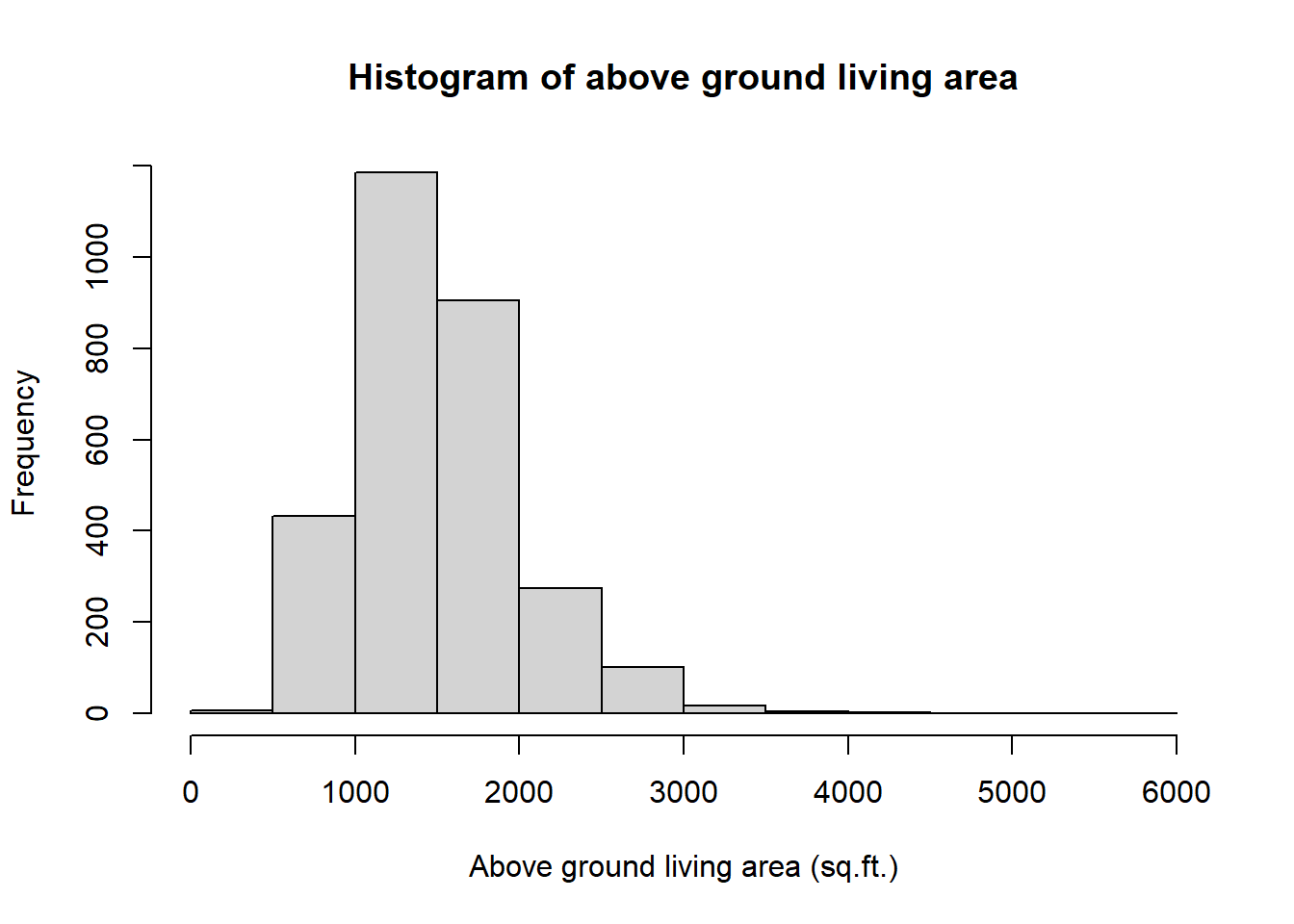
## 334 1126 1442 1500 1743 5642The above ground living area of the house variable contains 2930 distinct observations and there are not missing values. We see that the distribution of above ground living area of the house population variable has a mean of 1499.69 sq.ft.(square feet), a median of 1442 sq.ft. and a population standard deviation of 505.42 sq.ft. Observations in the dataset range from a minimum of 334sq.ft. for the smallest house to a maximum of 5642 sq.ft. for the biggest house. The histogram of the variable shows a positive (right) skew of the population data.
hist(area,
     main = "Histogram of above ground living area",
     xlab = "Above ground living area (sq.ft.)",
     )
In this exercise, we have access to the entire population of sales transactions, but this is rarely the case in real life. Gathering information on an entire population is often extremely costly or impossible. Because of this, we often take a sample of the population and use that to understand the properties of the population.
For our learning purpose, having the entire population of interest can help us understand the relation between population, samples, and sampling distribution. In this lab we will take smaller samples from the full population.
area <- ames$Gr.Liv.Area # create new dataset containing only variable 'Gr.Liv.Area' from dataset 'ames'

samp1 <- sample(area, 50) #take a random sample of 50 observations from the dataset 'area'

mean(samp1) # mean of the sample distribution for area. Note difference from population mean.
## [1] 1416.4
This command collects a simple random sample of size 50 from the ames dataset, which is assigned to samp1. This is like going into the City Assessor’s database and pulling up the files on 50 random home sales. Working with these 50 files would be considerably simpler than working with all 2930 home sales.
Exercise
Using your RStudio, take a sample, also of size 50, and call it
samp1. Take a second sample of size 1000, and call itsamp2. How does the mean ofsamp1compare with the mean ofsamp2?Suppose we took two more samples, one of size 1500 and another of size 2000. Which would you think would provide a more accurate estimate of the population mean?
Not surprisingly, every time we take another random sample, we get a different sample mean. It’s useful to get a sense of just how much variability we should expect when estimating the population mean this way. The distribution of sample means, called the sampling distribution, can help us understand this variability. In this lab, because we have access to the population, we can build up the sampling distribution of the sample mean by repeating the above steps many times (also called “drawing samples from the population”). Here we will generate 5000 samples of size 50 from the population, calculate the mean of each sample, and store each result in a vector called sample_means50. We will then plot the histogram of this sampling distribution.
area <- ames$Gr.Liv.Area
sample_means50 <- rep(NA, 5000) #initialise a vector

for(i in 1:5000){       # use of a loop function to draw a random sample 5000 times
   samp <- sample(area, 50)
   sample_means50[i] <- mean(samp)
}

hist(sample_means50, breaks = 25,
     main = "Sampling distribution of sample mean for Above ground living area",
     xlab = "Means (sq.ft.)") #Histogram of the 5000 samples (sampling distribution of the samples mean)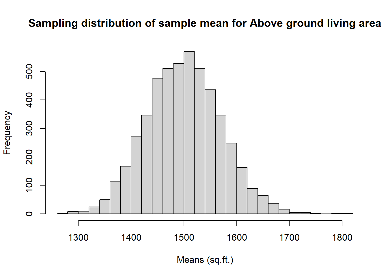
Try running the code a number of times. What do you observe? Each time you run the code, you see slightly different sampling distribution of mean.
What happens to the distribution if we instead collected 50,000 sample means? Try it! Change the number of draws on the code above and see how the shape of distribution changes.
(Hint: Check the normality of the distribution.)
4.1.1 Interlude: The for Loop
Let’s take a break from the statistics for a moment to let that last block of code sink in. You have just run your first for loop, a cornerstone of computer programming. The idea behind the for loop is iteration: it allows you to execute code as many times as you want without having to type out every iteration. In the case above, we wanted to iterate the two lines of code inside the curly braces that take a random sample of size 50 from area then save the mean of that sample into the sample_means50 vector. Without the for loop, this would be painful.
With the for loop, these thousands of lines of code are compressed into a handful of lines. We’ve added one extra line to the code below, which prints the mean of each sample drawn during each iteration of the for loop. Run this code.
sample_means50 <- rep(NA, 5000)
for(i in 1:5000){
samp <- sample(area, 50)
sample_means50[i] <- mean(samp)
print(sample_means50[i])
}
Let’s consider this code line by line to figure out what it does. In the first line we have initialised a vector. In this case, we created a vector of 5000 zeros called sample_means50. This vector will store values generated within the for loop.
The second line calls the for loop itself. The syntax can be loosely read as: “for every element i from 1 to 5000, run the following lines of code.” You can think of i as the counter that keeps track of which loop you’re on. Therefore, more precisely, the loop will run once when i = 1, then once when i = 2, and so on up to i = 5000.
The body of the for loop is the part inside the curly braces, and this set of code is run for each value of i. Here, on every loop, we take a random sample of size 50 from area, take its mean, and store it as the
\(i\)th element of sample_means50.
In order to display that this is really happening, we asked R to print print(sample_means50[i]) at each iteration. This line of code is optional and is only used for displaying what’s going on while the for loop is running.
The for loop allows us to not just run the code 5000 times, but to neatly package the results, element by element, into the empty vector that we initialised at the outset.
Exercise
To make sure you understand what you’ve done in this loop, try running a smaller version. Go to RStudio and initialise a vector of 100 zeros called sample_means_small. Run a loop that takes a sample of size 50 from area and stores the sample mean in sample_means_small, but only iterate from 1 to 100. Print the output to your screen (type sample_means_small into the console and press enter). How many elements are there in this object called sample_means_small? What does each element represent?
Solution:
area <- ames$Gr.Liv.Area
sample_means_small <- rep(0, 100)

for(i in 1:100){
   samp <- sample(area, 50)
   sample_means_small[i] <- mean(samp)
}

hist(sample_means_small, breaks = 25)
4.2 Sample Size and Sampling Distribution
Mechanics aside, let’s return to the reason we used a for loop in Sampling Distribution section: to compute a sampling distribution, specifically, this one.
area <- ames$Gr.Liv.Area
sample_means50 <- rep(NA, 5000)

for(i in 1:5000){
   samp <- sample(area, 50)
   sample_means50[i] <- mean(samp)
}

hist(sample_means50)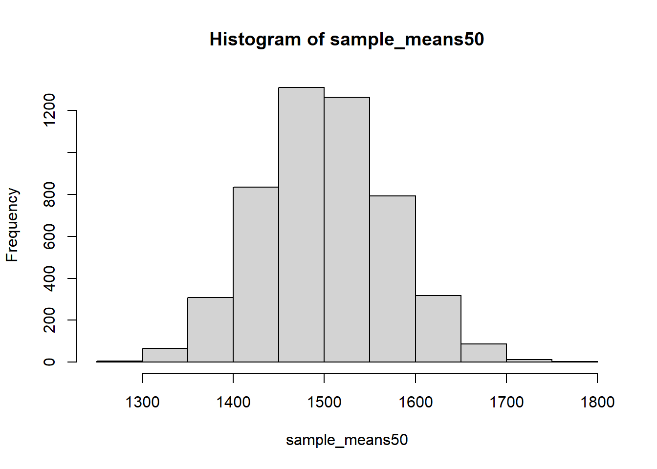
The sampling distribution that we computed tells us much about estimating the average living area in homes in Ames. Because the sample mean is an unbiased estimator, the sampling distribution is centred at the true average living area of the the population, and the spread of the distribution indicates how much variability is induced by sampling only 50 home sales.
To get a sense of the effect that sample size has on our distribution, let’s build up two more sampling distributions: one based on a sample size of 10 and another based on a sample size of 100 from a population size of 5000.
area <- ames$Gr.Liv.Area
sample_means10 <- rep(NA, 5000)
sample_means100 <- rep(NA, 5000)

for(i in 1:5000){
  samp <- sample(area, 10)
  sample_means10[i] <- mean(samp)
  samp <- sample(area, 100)
  sample_means100[i] <- mean(samp)
}
Here we’re able to use a single for loop to build two distributions by adding additional lines inside the curly braces. Don’t worry about the fact that samp is used for the name of two different objects. In the second command of the for loop, the mean of samp is saved to the relevant place in the vector sample_means10. With the mean saved, we’re now free to overwrite the object samp with a new sample, this time of size 100. In general, anytime you create an object using a name that is already in use, the old object will get replaced with the new one.
To see the effect that different sample sizes have on the sampling distribution, let’s plot the three distributions on top of one another.
area <- ames$Gr.Liv.Area
sample_means10 <- rep(NA, 5000)
sample_means50 <- rep(NA, 5000)
sample_means100 <- rep(NA, 5000)

for(i in 1:5000){
  samp <- sample(area, 10)
  sample_means10[i] <- mean(samp)
  samp <- sample(area, 50)
  sample_means50[i] <- mean(samp)
  samp <- sample(area, 100)
  sample_means100[i] <- mean(samp)
}

par(mfrow = c(3, 1))  # this creates 3 rows and 1 column for graphs

xlimits <- range(sample_means10)

hist(sample_means10,  breaks = 25, xlim = xlimits)
hist(sample_means50,  breaks = 25, xlim = xlimits)
hist(sample_means100, breaks = 25, xlim = xlimits)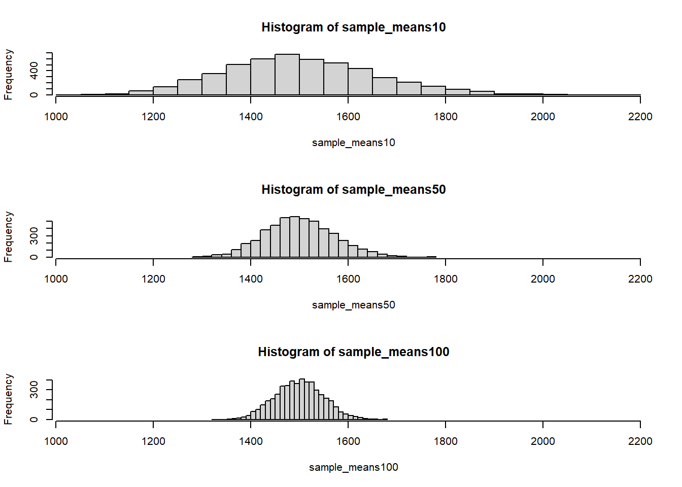
The first command specifies that you’d like to divide the plotting area into 3 rows and 1 column of plots (to return to the default setting of plotting one at a time, use par(mfrow = c(1, 1)). The breaks argument specifies the number of bins used in constructing the histogram. The xlim argument specifies the range of the x-axis of the histogram, and by setting it equal to xlimits for each histogram, we ensure that all three histograms will be plotted with the same limits on the x-axis. Here, I set it to be the same as the histogram which has more spread on the x-axis.
Your turn! Try different sample sizes and see what happens to the distribution.
- When the sample size is larger, what happens to the center? What about the spread?
- The center moves to the right; standard deviation gets smaller
- The center approaches to the true mean; the standard deviation does not change
- The center approaches to the true mean; the standard deviation gets smaller
Exercise So far, we have only focused on estimating the mean living area in homes in Ames. Now you’ll try to estimate the mean home price and do the same analyses we did above for living area using RStudio. Specifically,
Take a random sample of size 50 from
price. Using this sample, what is your best point estimate of the population mean?Since you have access to the population, simulate the sampling distribution for \(\bar{x}_{price}\) by taking 5000 samples from the population of size 50 and computing 5000 sample means. Store these means in a vector called
sample_means50. Plot the data, then describe the shape of this sampling distribution. Based on this sampling distribution, what would you guess the mean home price of the population to be? Finally, calculate and report the population mean.Change your sample size from 50 to 1500, then compute the sampling distribution using the same method as above, and store these means in a new vector called
sample_means1500. Describe the shape of this sampling distribution, and compare it to the sampling distribution for a sample size of 50. Based on this sampling distribution, what would you guess to be the mean sale price of homes in Ames?Of the sampling distributions from 2 and 3, which has a smaller spread? If we’re concerned with making estimates that are more often close to the true value, would we prefer a distribution with a large or small spread?
4.3 Hypothesis Testing
4.3.1 The Data
In this exercise, we use a dataset from North Carolina, USA. In 2004, the state of North Carolina released a large data set containing information on births recorded in this state. This data set is useful to researchers studying the relation between the habits and practices of expectant mothers and the birth of their children. We will work with a random sample of observations from this data set, which we call nc.
We have observations on 13 different variables, some categorical and some numerical. The meaning of each variable is as follows.
| Variable | Description |
|---|---|
fage |
father’s age in years. |
mage |
mother’s age in years. |
mature |
maturity status of mother. |
weeks |
length of pregnancy in weeks. |
premie |
whether the birth was classified as premature (premie) or full-term. |
visits |
number of hospital visits during pregnancy. |
marital |
whether mother is married or not married at birth. |
gained |
weight gained by mother during pregnancy in pounds. |
weight |
weight of the baby at birth in pounds. |
lowbirthweight |
whether baby was classified as low birthweight (low) or not (not low). |
gender |
gender of the baby, female or male. |
habit |
status of the mother as a nonsmoker or a smoker. |
whitemom |
whether mother is white or not white. |
4.3.2 Exploratory analysis
Before undertaking any hypothesis testing, we need to understand the data and perform explanatory analysis.
nc <- read.csv("http://bit.ly/31adfCe")
glimpse(nc) # just glimpse of how the data looks like
## Rows: 1,000
## Columns: 13
## $ fage <int> NA, NA, 19, 21, NA, NA, 18, 17, NA, 20, ~
## $ mage <int> 13, 14, 15, 15, 15, 15, 15, 15, 16, 16, ~
## $ mature <chr> "younger mom", "younger mom", "younger m~
## $ weeks <int> 39, 42, 37, 41, 39, 38, 37, 35, 38, 37, ~
## $ premie <chr> "full term", "full term", "full term", "~
## $ visits <int> 10, 15, 11, 6, 9, 19, 12, 5, 9, 13, 9, 8~
## $ marital <chr> "married", "married", "married", "marrie~
## $ gained <int> 38, 20, 38, 34, 27, 22, 76, 15, NA, 52, ~
## $ weight <dbl> 7.63, 7.88, 6.63, 8.00, 6.38, 5.38, 8.44~
## $ lowbirthweight <chr> "not low", "not low", "not low", "not lo~
## $ gender <chr> "male", "male", "female", "male", "femal~
## $ habit <chr> "nonsmoker", "nonsmoker", "nonsmoker", "~
## $ whitemom <chr> "not white", "not white", "white", "whit~summary(nc) # summary of the data## fage mage mature weeks
## Min. :14.00 Min. :13 Length:1000 Min. :20.00
## 1st Qu.:25.00 1st Qu.:22 Class :character 1st Qu.:37.00
## Median :30.00 Median :27 Mode :character Median :39.00
## Mean :30.26 Mean :27 Mean :38.33
## 3rd Qu.:35.00 3rd Qu.:32 3rd Qu.:40.00
## Max. :55.00 Max. :50 Max. :45.00
## NA's :171 NA's :2
## premie visits marital
## Length:1000 Min. : 0.0 Length:1000
## Class :character 1st Qu.:10.0 Class :character
## Mode :character Median :12.0 Mode :character
## Mean :12.1
## 3rd Qu.:15.0
## Max. :30.0
## NA's :9
## gained weight lowbirthweight
## Min. : 0.00 Min. : 1.000 Length:1000
## 1st Qu.:20.00 1st Qu.: 6.380 Class :character
## Median :30.00 Median : 7.310 Mode :character
## Mean :30.33 Mean : 7.101
## 3rd Qu.:38.00 3rd Qu.: 8.060
## Max. :85.00 Max. :11.750
## NA's :27
## gender habit whitemom
## Length:1000 Length:1000 Length:1000
## Class :character Class :character Class :character
## Mode :character Mode :character Mode :character
##
##
##
## As you review the variable summaries, consider which variables are categorical and which are numerical. For numerical variables, are there outliers? The best way to see this is by plotting the data.
In the 2004 North Carolina birth dataset we have a total of 1000 observations and 13 variables; 7 are categorical (mature, habit, whitemom, premie, marital, lowbirthweight, gender), 6 numerical (fage, mage, weeks, visits, gained, weigh). In this case we consider the possible relationship between a mother’s smoking habit and the weight of her baby for smokers and for non-smokers. Our variables of interest are
- habit - status of the mother as a non-smoker or a smoker
- weight - weight of the baby at birth in pounds.
In this dataset the recorded weight of babies at birth range from a minimum of 1 pound to a maximum of 11.75 pounds with a mean weight of 7.10 pounds and standard deviation of 1.51 pounds. The variable doesn’t contain missing values.
The variable habit, contain 1 missing values and divides the sample in 2 groups: smokers (126 observations) and non-smokers (873 observations) for a total of 999 valid observations. Note: In general observations with missing values should be examined and eventually removed or dealt with. In this exercise we will just ignore it for now but will consider it during the hypothesis test.
Plotting the data is a useful first step because it helps us quickly visualise trends, identify strong associations, and develop research questions.
So, let’s make a side-by-side boxplot of habit and weight for smokers and non-smokers using ggplot. What does the plot highlight about the relationship between these two variables?
ggplot(data = na.omit(nc),
  aes(x = habit, y = weight, colour = habit))  +
  geom_boxplot() + xlab("Smoking Habit")      +
  ylab("Baby's Weight")                       +
  ggtitle("Mother's Habit vs baby's Weight")  +
stat_summary(fun = mean, colour = "darkred", geom = "point", shape = 1, size = 3) 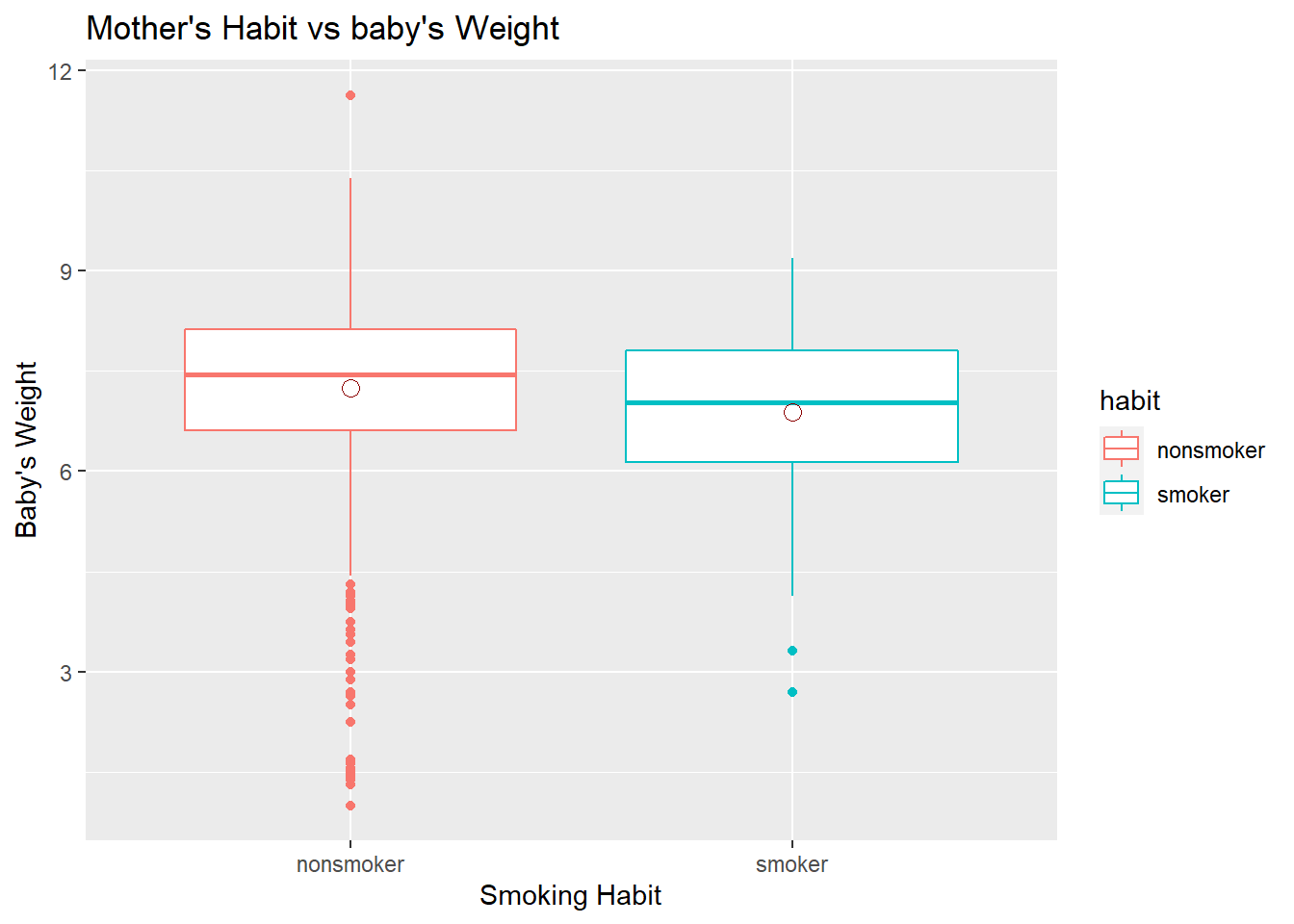
The box plots show how the medians of the two distributions compare, but we can also compare the means of the distributions which the last line in that code does by adding the means on boxplot using stat_summary(). We see some differences in means, but is this difference statistically significant? In order to answer this question, we will conduct a hypothesis test.
Exercise:
Go to Rstudio and try producing the same plot above using R Base function boxplot().
Solution:
data = na.omit(nc)
boxplot(data$weight ~ data$habit ,
        main = "Mother's Habit vs baby's Weight",
        ylab = "Baby's Weight",
        xlab = "Smoking Habit",
        col = c("red", "green")
       )
legend("topleft", c("nonsmoker", "smoker"), fill = c("red", "green"))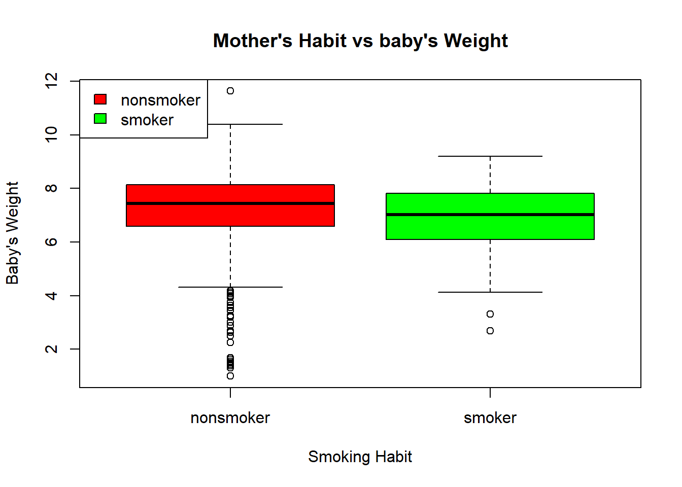
4.3.3 Inference
Before we perform a hypothesis test, we need to check if the conditions necessary for inference are satisfied. Note that you will need to obtain sample sizes to check the conditions and check the outliers. You can compute the group size using by(nc$weight, nc$habit, length). You can continue on the code above to find out the number of observations in smoker and non-smoker groups.
Once we check the data, the next step is to write the hypotheses for testing if the average weights of babies born to smoking and non-smoking mothers are different.
To undertake the testing, we will use a function called inference. This function will allow us to conduct hypothesis tests and construct confidence intervals. You need to install “statsr” package to be able to use inference()
statsr::inference(y = weight, x = habit, data = nc,
          statistic = c("mean"),
          type = c("ci"),
          null = 0,
          alternative = c("twosided"),
          method = c("theoretical"),
          conf_level = 0.95,
          order = c("smoker","nonsmoker"))
## Response variable: numerical, Explanatory variable: categorical (2 levels)
## n_smoker = 126, y_bar_smoker = 6.8287, s_smoker = 1.3862
## n_nonsmoker = 873, y_bar_nonsmoker = 7.1443, s_nonsmoker = 1.5187
## 95% CI (smoker - nonsmoker): (-0.5803 , -0.0508)
Let’s pause for a moment to go through the arguments of this custom function. The first argument is y, which is the response variable that we are interested in: nc$weight. The second argument is the explanatory variable, x, which is the variable that splits the data into two groups, smokers and non-smokers: nc$habit. The argument, est, is the parameter we’re interested in: "mean" (other options are "median", or "proportion"). Next we decide on the type of inference we want: a hypothesis test ("ht") or a confidence interval ("ci"). When performing a hypothesis test, we also need to supply the null value, which in this case is 0, since the null hypothesis sets the two population means equal to each other. The alternative hypothesis can be "less", "greater", or "twosided". The method of inference can be "theoretical" or "simulation" based. Here, we use theoretical one using an existing dataset. To set the confidence level, we use conf_level. By default the function reports an interval for (\(\mu_{nonsmoker} - \mu_{smoker}\)). We can easily change this order by using the order argument.
Let’s run this code.
data = na.omit(nc) # let's omit missing values from our calculations

inference(y = weight, x = habit, data = data,
          statistic = c("mean"),
          type = c("ci"),
          null = 0,
          alternative = c("twosided"),
          method = c("theoretical"),
          conf_level = 0.95,
          order = c("smoker","nonsmoker"))
## Response variable: numerical, Explanatory variable: categorical (2 levels)
## n_smoker = 84, y_bar_smoker = 6.8864, s_smoker = 1.3064
## n_nonsmoker = 716, y_bar_nonsmoker = 7.2468, s_nonsmoker = 1.4521
## 95% CI (smoker - nonsmoker): (-0.6637 , -0.057)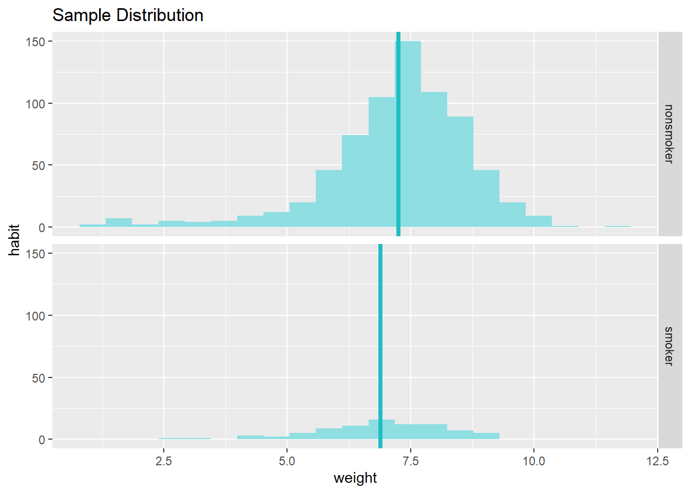
From these two plots, we can see that there are some differences in the measurement of central tendency and spread. Your output also provides confidence intervals for the difference between means of smokers and non-smokers. As the confidence interval does not include the null value (i.e., 0), we can say that the difference we observe is statistically significant and different from zero. We could perform a hypothesis test (in this case a t-test) to see this. We just need to specify the type to "ht" in the command demonstrated below:
For a t-test:
data = na.omit(nc) # let's omit missing values from our calculations

inference(y = weight, x = habit, data = data,
          statistic = c("mean"),
          type = c("ht"),
          null = 0,
          alternative = c("twosided"),
          method = c("theoretical"),
          conf_level = 0.95,
          order = c("smoker","nonsmoker"))
## Response variable: numerical
## Explanatory variable: categorical (2 levels)
## n_smoker = 84, y_bar_smoker = 6.8864, s_smoker = 1.3064
## n_nonsmoker = 716, y_bar_nonsmoker = 7.2468, s_nonsmoker = 1.4521
## H0: mu_smoker = mu_nonsmoker
## HA: mu_smoker != mu_nonsmoker
## t = -2.3625, df = 83
## p_value = 0.0205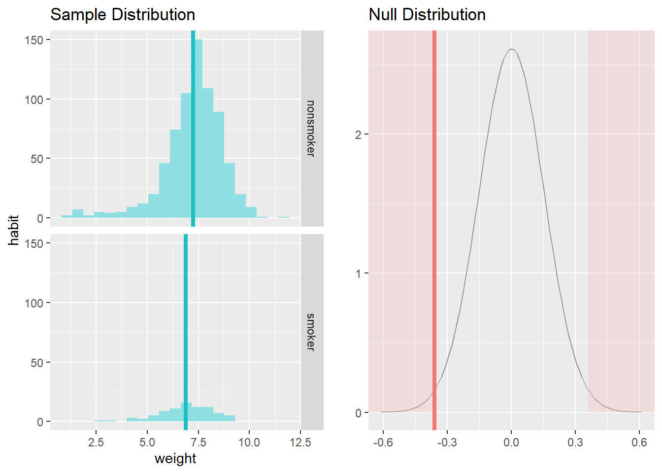
If you run this command, you will see that the t-value is -2.36 and p-value is less than alpha = 0.05, so we can conclude the same result about the significance of the difference between means.