Chapter 2 Data Basics
Well done! You have completed your Session 1 and are now ready to explore the data using R. In this section, we will learn how to load the data, and investigate variables in a dataset, as well as how to export and save the data in different formats.
2.1 Loading Data
There are two ways you can load the data to R: (1) using the weblink of the dataset provided to you or (2) opening the dataset from a file already saved in your computer. In almost all exercises, I will provide you the links for the datasets you will use in practice exercises and assessed questions. For both methods, the typical data file extension we use is an Excel csv file.
NOTE 1: If you are wondering where your files and data are saved in your computer, you can simply find the working directory by typing: getwd() on the R console. You can change this working directory as follows:
- Let’s create a sub-directory named “R” in your “Documents” folder, which you will use for your R-practicals.
- From RStudio, use the menu to change your working directory under
Session > Set Working Directory > Choose Directory. - Choose the directory you have just created in step 1
It’s also possible to use the R function setwd(), which stands for “set working directory.”
- For Mac: e.g.,
setwd("/path/to/my/directory") - For Windows: e.g.,
setwd("c:/Documents/my/working/directory")with an extension of the full address of the folder.
2.1.1 The Data
The data we will use in this section is from the British Household Panel Survey (BHPS) – a longitudinal household survey administered by the University of Essex, UK. A sample of British households was drawn and first interviewed in 1991. The members of these original households have since been followed and annually interviewed. Each wave contains information on individuals aged 15 and over who were enumerated in the household. In this practical, we will use the reduced version of the first wave of the BHPS.
The data file is in csv format and called bhps and can be accessed using the link provided below. After loading the data, we will have a look at it as well.
You can load the data using one of the following options in your RStudio:
read.csv(): R’s basic function
bhps <- read.csv("http://bit.ly/2ybNWDk")read_csv(): An option faster with the big data. For this, you need to installtidyversepackage first.
# Check if package Tidyverse is already installed and if not it will install it
if("tidyverse" %in% rownames(installed.packages()) == FALSE) {install.packages("tidyverse")}
#Load library Tidyverse
library(tidyverse)

# Load the dataset
bhps <- read_csv("http://bit.ly/2ybNWDk")
Both options work.
Note 1: if this csv data file was in a folder in your PC, you would have loaded the file by typing: bhps <- read_csv("..where the data file is in your PC.."). For example, you might have saved the data file in a folder called Statistics on your desktop. In that case, the address of the data file would look like this: "C:/Desktop/Statistics/bhps.csv". Don’t forget to include the quotation marks " " around the file address in your code.
You could also import (or load) a data file in other Excel file format, rather than csv, such as xls. In that case, you need to use read.xls() instead. For this, you need to install openxlsx() package. We will not be using this format in this module. In fact, it is not too common.
Note 2: The dataset includes 10258 observations (rows). Instead of showing all rows, we can have a look at the first 6 rows by typing head(bhps):
head(bhps)## # A tibble: 6 x 7
## id female region academic_qual dob age numchild
## <dbl> <dbl> <chr> <chr> <dbl> <dbl> <dbl>
## 1 1 1 london None 1899 91 0
## 2 2 0 london Degree + 1963 28 0
## 3 3 0 london Degree + 1965 26 0
## 4 4 1 london GCSE/CSE/OLevel 1933 58 0
## 5 5 1 london None 1937 54 0
## 6 6 0 london Degree + 1934 57 0This head() function is very handy when you have large datasets.
Remember, most data (csv-files, Excel sheets) is organised in 2 dimensional fashion and can be read directly into dataframes. Here, the dataset bhps is stored in a dataframe called bhps. To see the structure of this dataframe, we just use the str(). Go back to RStudio, and try this function and see the structure of the bhps dataset. Don’t forget to load the data first!
In this dataset, the column (i.e., variable) names are assigned. Sometimes, the data might not have column names. In that case, you can use col_names = FALSE to tell read_csv() not to treat the first row as headings, and instead label them sequentially from \(x_1\) to \(x_n\). For example:
read_csv("1,2,3\n4,5,6", col_names = FALSE)## # A tibble: 2 x 3
## X1 X2 X3
## <dbl> <dbl> <dbl>
## 1 1 2 3
## 2 4 5 6Here, we are creating a small csv file. \n is a convenient shortcut for adding a new line.
Alternatively you can pass col_names a character vector which will be used as the column names:
read_csv("1,2,3\n4,5,6", col_names = c("x", "y", "z"))## # A tibble: 2 x 3
## x y z
## <dbl> <dbl> <dbl>
## 1 1 2 3
## 2 4 5 6Another option that commonly needs tweaking is na: this specifies the value (or values) that are used to represent missing values in your file:
read_csv("1,2,3\n4,5,.", col_names = c("x", "y", "z"), na = ".")## # A tibble: 2 x 3
## x y z
## <dbl> <dbl> <dbl>
## 1 1 2 3
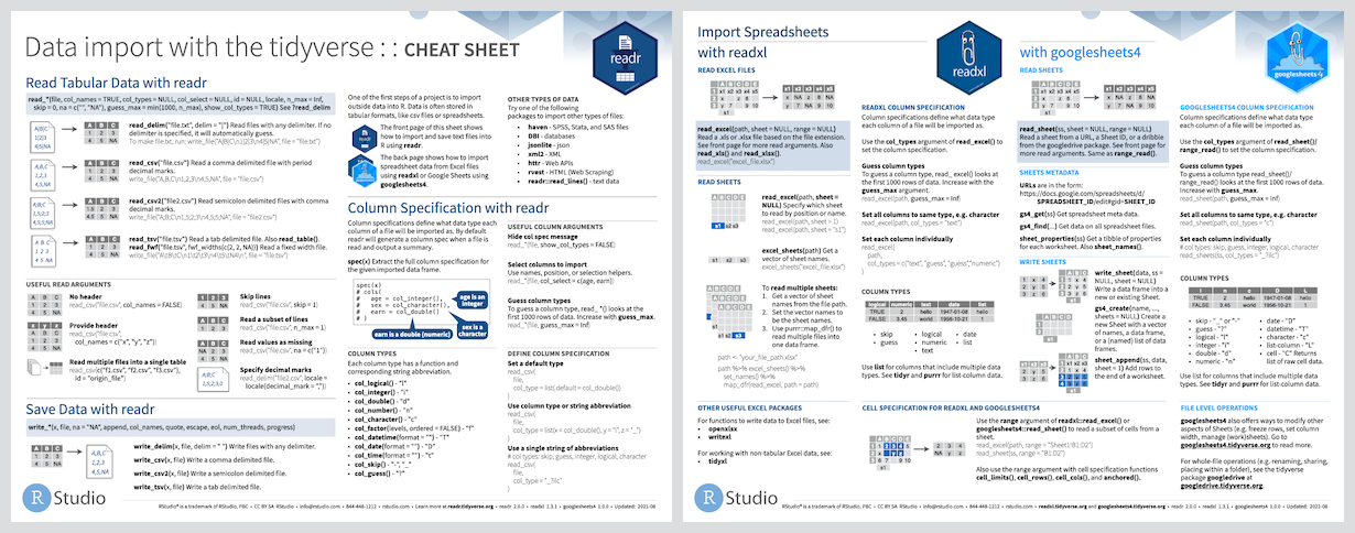
## 2 4 5 NAThe following table shows the most useful R functions used for importing (loading) certain types of data. We may not use them all, but I am just summarising them here for your information. Some file formats will be discussed in the “Exporting Data” section.
| import file type | R function to use to open the file |
|---|---|
| .txt | read.table() |
| .csv | read.csv() and readr::read_csv() (easiest way to get readr is to install the whole tidyverse package) |
| .xlx and .xlsx | readxl::read_excel() and openxlsx::read.xlsx() |
| .Rdata or rda | load() |
| .rds | read.RDS() and read_rds() |
| Internet | download.file() |
Here, a double semicollon :: is used to access a package (e.g., readr) to run the function following it. Simply type in package::function_name. Type and run ? "::" to learn more about double semicollon.
2.2 Exporting Data
Although getting data into R is essential, getting data out of R can be just as important. Whether you need to export data or analytic results simply to store, share, or feed into another system it is generally a straightforward process.
In this section, we will learn how to export data to text files, Excel files, and save to R data objects.
I will start demonstrating how to do things using the commonly used base R functions, then I will cover functions from the popular readr and xlsx packages.
2.2.1 Exporting to a text file
We can export the data in text format using: (1) base R functions or (2) readr package functions.
Base R functions:
We use write.table() function in base R for exporting the data. The functions write.csv() and write.delim() are special cases of write.table(). Let me demonstrate how to use them below. First, let’s create a dataframe which has numeric, string (character) and logical types of data.
df <- data.frame(var1 = c(10, 25, 8),
                 var2 = c("beer", "wine", "cheese"),
                 var3 = c(TRUE, TRUE, FALSE),
                 row.names = c("billy", "bob", "thornton"))

df
## var1 var2 var3
## billy 10 beer TRUE
## bob 25 wine TRUE
## thornton 8 cheese FALSETo export df to a .csv file we can use write.csv(). Additional arguments allow you to exclude row and column names, specify what to use for missing values, add or remove quotations around character strings, etc.
write to a csv file
write.csv(df, file = "C:/.../export_csv")write to a csv file with added arguments
write.csv(df, file = "C:/.../export_csv", row.names = FALSE, na = "MISSING!")
In addition to .csv files, we can also write to other text files using write.table.
write.table(df, file = "C:/.../export_txt", sep="\t")
readr package:
The readr package uses write functions similar to base R. However, readr write functions are about twice as fast and they do not write row names. One thing to note, where base R write functions use the file = argument, readr write functions use path = or file = depending on the version installed. col_names = TRUE asks to add the column names at the top of the file. If you don’t want it, then use FALSE.
library(readr)

df <- data.frame(var1 = c(10, 25, 8),
                 var2 = c("beer", "wine", "cheese"),
                 var3 = c(TRUE, TRUE, FALSE),
                 row.names = c("billy", "bob", "thornton"))

# write to a csv file
write_csv(df, path = "export_csv1.csv")

# write to a csv file without column names
write_csv(df, path = "export_csv2.csv", col_names = TRUE)
Exercise: Can you export the bhps data we studied earlier to your working folder as a csv file called bhps_exported.csv?
2.2.2 Exporting to Excel files
You can export the data to Excel files using:
readrpackagexlsxpackage
There are possibly some other ways of exporting the data, but I will just focus on these two for now.
So, let me provide the basic codes for these two techniques now.
readr package
library(readr)

df <- data.frame(var1 = c(10, 25, 8),
                 var2 = c("beer", "wine", "cheese"),
                 var3 = c(TRUE, TRUE, FALSE),
                 row.names = c("billy", "bob", "thornton"))

write_excel_csv(df, path = "df.csv", col_names = FALSE)
xlsx package
df <- data.frame(var1 = c(10, 25, 8),
                 var2 = c("beer", "wine", "cheese"),
                 var3 = c(TRUE, TRUE, FALSE),
                 row.names = c("billy", "bob", "thornton"))

# install the openxlsx package first. Only do once.
library(openxlsx)

# write to a .xlsx file
write.xlsx(df, file = "output_example.xlsx")

# write to a .xlsx file without row names
write.xlsx(df, file = "output_example.xlsx", row.names = FALSE)
Note: Typically, we work with csv files, so you will be exporting your data into csv file if required.
Exercise: Can you export the bhps data we studied earlier to your working folder as a xlsx file called bhps_exported.xlsx?
2.2.3 Exporting R object files
Sometimes you may need to save data or other R objects outside of your workspace. You may want to share R data/objects with co-workers, transfer between projects or computers, or simply archive them. There are three primary ways that people tend to save R data/objects: as .RData, .rda, or as .rds files.
.rda is just short for .RData, therefore these file extensions represent the same underlying object type. You use the .rda or .RData file types when you want to save several, or all, objects and functions that exist in your “global environment.” On the other hand, if you only want to save a single R object such as a data frame, function, or statistical model results it is best to use .rds file type. You can use .rda or .RData to save a single object but the benefit of .rds is it only saves a representation of the object and not the name whereas .rda and .RData save the both the object and its name. As a result, with .rds the saved object can be loaded into a named object within R that is different from the name it had when originally saved. The following illustrates how you save R objects with each type.
# save() can be used to save multiple objects in your global environment.

# lets save two objects to a .RData file
x <- c(1:20)
y <- list(a = 1, b = TRUE, c = "oops")
save(x, y, file = "xy.RData")

# save.image() is just a short-cut for ‘save my current workspace’,
# i.e. all objects in your global environment
save.image()

# write rds file using readr package
readr::write_rds(x, "x.rds")

# save a single object to file
saveRDS(x, "x.rds")

# restore it under a different name
x2 <- readRDS("x.rds")

# See if c=x and x2 are identical
identical(x, x2)
The following table is a summary of the useful R functions used for exporting certain types of data. We may not use them all in this course, but I am just listing them here for you to practise.
| export file type | R function to use to export the file |
|---|---|
| .txt | write.table() |
| .csv | write.csv() and readr::write_csv() |
| .xlx and .xlsx | xlsx::write.xlsx() |
| .Rdata or rda | save(data1, data2, file = "filename.rda") |
| .rds | readr::write_rds() |
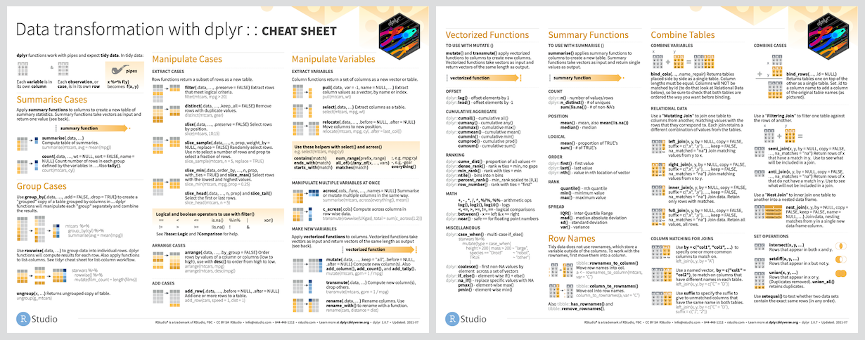
2.3 Data Transformation by dplyr
2.3.1 What is dplyr?
dplyr is a type of grammar used for data manipulation, providing a consistent set of verbs that help you solve the most common data manipulation challenges:
mutate()adds new variables that are functions of existing variablesselect()picks variables based on their names.filter()picks cases based on their values.group_by()groups data by categorical levelssummarise()reduces multiple values down to a single summary.arrange()changes the ordering of the rows.join()joins separate dataframes
You can learn more about them in vignette("dplyr"). As well as these single-table verbs, dplyr also provides a variety of two-table verbs, which you can learn about in vignette("two-table").
2.3.2 Installation
The easiest way to get dplyr is to install the whole tidyverse package:
install.packages("tidyverse", dependencies = TRUE)Here dependencies= TRUE ensures package dependencies (i.e., what other packages the one you are installing needs to work) are also installed. It is not mandatory to include it, but is a nice practice to make sure all you need is installed.
Alternatively, we can install just dplyr:
install.packages("dplyr", dependencies = TRUE)2.3.4 Interlude: Pipe %>% operator
This operator will forward a value, or the result of an expression, into the next function call/expression. It can be interpreted as “and then”. In order to use this, you need to install dplry package.
2.3.5 mutate() function
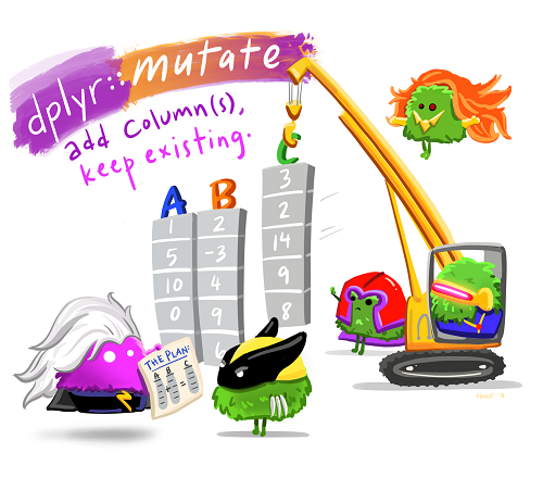
Figure 2.1: Designed by Allison Horst
This function creates a new variable. In the exercise below, let’s create a new variable called “new_age” using the “age” variable from the bhps data. This new variable is just “age + 2.”
new_data <- bhps %>% mutate(new_age = age + 2)
head(new_data)
2.3.6 select() function
The aim is to reduce the dataframe size to only desired variables. This is usually very practical when you have large datasets and you just need to access specific variables.
Let’s select only 4 variables (id, female, region, and age) from bhps dataset and view the first 6 observations using head(bhps). Remember that you can download the data from http://bit.ly/2ybNWDk if you haven’t done so. If you already loaded the data, you don’t need to do it again.
new_data <- bhps %>% select(id, female, region, age)
head(new_data)
## # A tibble: 6 x 4
## id female region age
## <dbl> <dbl> <chr> <dbl>
## 1 1 1 london 91
## 2 2 0 london 28
## 3 3 0 london 26
## 4 4 1 london 58
## 5 5 1 london 54
## 6 6 0 london 57You can also deselect by using - prior to name or function. The following produces the inverse of the function above.
new_data <- bhps %>% select(-academic_qual, -dob, -numchild)
head(new_data)
## # A tibble: 6 x 4
## id female region age
## <dbl> <dbl> <chr> <dbl>
## 1 1 1 london 91
## 2 2 0 london 28
## 3 3 0 london 26
## 4 4 1 london 58
## 5 5 1 london 54
## 6 6 0 london 57There are some special functions of the select() function. To view these and if you want to know more about the select() function, just run ? select().
2.3.7 filter() function
The aim is to reduce rows/observations with matching conditions. Let’s identify cases for female participants.
new_data <- bhps %>% filter(female == 1)
head(new_data)
## # A tibble: 6 x 7
## id female region academic_qual dob age numchild
## <dbl> <dbl> <chr> <chr> <dbl> <dbl> <dbl>
## 1 1 1 london None 1899 91 0
## 2 4 1 london GCSE/CSE/OLevel 1933 58 0
## 3 5 1 london None 1937 54 0
## 4 8 1 london <NA> 1959 32 1
## 5 9 1 london Degree + 1942 49 1
## 6 11 1 london None 1932 59 0We can apply multiple logic rules in the filter() function such as:
< Less than
> Greater than
== Equal to
<= Less than or equal to
>= Greater than or equal to
!= Not equal to
%in% Group membership
is.na is NA
!is.na is not NA
&, |, ! Boolean operators
For instance we can filter bhps for females over 18 years old.
new_data <- bhps %>% filter(female == 1 & age > 18)
head(new_data)
## # A tibble: 6 x 7
## id female region academic_qual dob age numchild
## <dbl> <dbl> <chr> <chr> <dbl> <dbl> <dbl>
## 1 1 1 london None 1899 91 0
## 2 4 1 london GCSE/CSE/OLevel 1933 58 0
## 3 5 1 london None 1937 54 0
## 4 8 1 london <NA> 1959 32 1
## 5 9 1 london Degree + 1942 49 1
## 6 11 1 london None 1932 59 02.3.8 group_by() function
The aim is to group data by categorical variables. The group_by() is a silent function in which no observable manipulation of the data is performed as a result of applying the function. Rather, the only change you’ll notice is, if you print the dataframe underneath the source information and prior to the actual dataframe, an indicator of what variable the data is grouped by will be provided. The real magic of the group_by() function comes when we perform summary statistics, which we will cover later.
new_data <- bhps %>% group_by(region)
head(new_data)
## # A tibble: 6 x 7
## # Groups: region [1]
## id female region academic_qual dob age numchild
## <dbl> <dbl> <chr> <chr> <dbl> <dbl> <dbl>
## 1 1 1 london None 1899 91 0
## 2 2 0 london Degree + 1963 28 0
## 3 3 0 london Degree + 1965 26 0
## 4 4 1 london GCSE/CSE/OLevel 1933 58 0
## 5 5 1 london None 1937 54 0
## 6 6 0 london Degree + 1934 57 02.3.9 summarise() function
This performs summary statistics, which we will use in next session. The summarise() function allows us to perform the majority of the initial summary statistics when performing exploratory data analysis.
bhps %>% summarise(  Min = min(age, na.rm = TRUE),
                     Median = median(age, na.rm = TRUE),
                     Mean = mean(age, na.rm = TRUE),
                     Var = var(age, na.rm = TRUE),
                     SD = sd(age, na.rm = TRUE),
                     Max = max(age, na.rm = TRUE),
                     N = n())
## # A tibble: 1 x 7
## Min Median Mean Var SD Max N
## <dbl> <dbl> <dbl> <dbl> <dbl> <dbl> <int>
## 1 15 42 44.5 341. 18.5 97 10258We will revisit this in “Descriptive Statistics” lecture. So, don’t worry if you don’t understand the summary statistics yet.
2.3.10 arrange() function
The aim is to order variable values. The arrange() function allows us to order data by variables in ascending or descending order.
Let’s arrange the dataset by region and for each region let’s order the age in increasing order.
Note: We can use pipe operator (%>%) to combine more than one manipulation.
bhps %>% group_by(region) %>%
         arrange(age)
## # A tibble: 10,258 x 7
## # Groups: region [11]
## id female region academic_qual dob age numchild
## <dbl> <dbl> <chr> <chr> <dbl> <dbl> <dbl>
## 1 10171 0 scotland GCSE/CSE/OLevel 1975 15 2
## 2 96 1 london None 1975 16 1
## 3 360 0 london GCSE/CSE/OLevel 1975 16 2
## 4 434 1 london GCSE/CSE/OLevel 1975 16 0
## 5 592 0 london GCSE/CSE/OLevel 1975 16 1
## 6 638 0 london GCSE/CSE/OLevel 1975 16 3
## 7 644 1 london GCSE/CSE/OLevel 1975 16 2
## 8 692 0 london GCSE/CSE/OLevel 1975 16 0
## 9 738 0 london GCSE/CSE/OLevel 1975 16 1
## 10 740 0 london None 1975 16 1
## # ... with 10,248 more rowsThe default ordering is “increasing,” we can specify the ordering to be “descending” within each region:
bhps %>% group_by(region) %>%
         arrange(desc(age))
## # A tibble: 10,258 x 7
## # Groups: region [11]
## id female region academic_qual dob age numchild
## <dbl> <dbl> <chr> <chr> <dbl> <dbl> <dbl>
## 1 9989 1 scotland None 1894 97 0
## 2 2416 1 south east None 1895 96 0
## 3 9187 0 wales <NA> 1897 94 0
## 4 299 1 london None 1898 93 0
## 5 990 1 london None 1898 93 0
## 6 2117 1 south east <NA> 1898 93 0
## 7 2466 1 south east None 1898 93 0
## 8 4896 1 east midlands None 1898 93 0
## 9 6146 1 north west <NA> 1898 93 0
## 10 7729 1 yorkshire & h~ <NA> 1899 92 0
## # ... with 10,248 more rows2.3.11 join() function
This joins two dataframes together. The different join functions control what happens to rows that exist in one table but not the other.
inner_joinkeeps only the entries that are present in both tables. inner_join is the only function that guarantees you won’t generate any missing entries.left_joinkeeps all the entries that are present in the left (first) table and excludes any that are only in the right table.right_joinkeeps all the entries that are present in the right table and excludes any that are only in the left table.full_joinkeeps all of the entries in both tables, regardless of whether or not they appear in the other table.
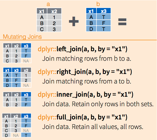
Figure 2.2: dplyr joins, via RStudio
Let’s practise.
# dataframe 1
a <- data.frame(x1 = c("A", "B", "C"), x2 = c(1,2,3))
a
##   x1 x2
## 1  A  1
## 2  B  2
## 3  C  3
#dataframe 2
b <- data.frame(x1 = c("A", "B", "D"), x3 = c("T", "F", "T"))
b
##   x1 x3
## 1  A  T
## 2  B  F
## 3  D  T
inner_join(a, b)
## Joining, by = "x1"
##   x1 x2 x3
## 1  A  1  T
## 2  B  2  F
As you see, inner_join() keeps rows appearing in both dataframes.
# dataframe 1
a <- data.frame(x1 = c("A", "B", "C"), x2 = c(1,2,3))
a
##   x1 x2
## 1  A  1
## 2  B  2
## 3  C  3
#dataframe 2
b <- data.frame(x1 = c("A", "B", "D"), x3 = c("T", "F", "T"))
b
##   x1 x3
## 1  A  T
## 2  B  F
## 3  D  T
left_join(a, b)
## Joining, by = "x1"
##   x1 x2   x3
## 1  A  1    T
## 2  B  2    F
## 3  C  3 <NA>
left_join() includes all rows appearing in the first (left) dataframe (i.e., a), and excludes any that are only in the second (right) dataframe (i.e., b).
# dataframe 1
a <- data.frame(x1 = c("A", "B", "C"), x2 = c(1,2,3))
a
##   x1 x2
## 1  A  1
## 2  B  2
## 3  C  3
#dataframe 2
b <- data.frame(x1 = c("A", "B", "D"), x3 = c("T", "F", "T"))
b
##   x1 x3
## 1  A  T
## 2  B  F
## 3  D  T
right_join(a, b)
## Joining, by = "x1"
##   x1 x2 x3
## 1  A  1  T
## 2  B  2  F
## 3  D NA  T
right_join() includes all rows appearing in the second (right) dataframe (i.e., b), and excludes any that are only in the first (left) dataframe (i.e., a).
# dataframe 1
a <- data.frame(x1 = c("A", "B", "C"), x2 = c(1,2,3))
a
##   x1 x2
## 1  A  1
## 2  B  2
## 3  C  3
#dataframe 2
b <- data.frame(x1 = c("A", "B", "D"), x3 = c("T", "F", "T"))
b
##   x1 x3
## 1  A  T
## 2  B  F
## 3  D  T
full_join(a, b)
## Joining, by = "x1"
##   x1 x2   x3
## 1  A  1    T
## 2  B  2    F
## 3  C  3 <NA>
## 4  D NA    T
full_join() includes all rows from both dataframes, regardless of whether or not they appear in the other dataframe.
Sometimes, the dataframes or tables that you want to combine may be in different sizes and may have different variables, as well as some overlapping variables. For example,
# dataframe 1
df1 <- data.frame(name = c("John", "Paul", "George", "Liz", "Danny"),
                  instrument = c("guitar", "bass", "drums", "bass", "guitar"))
df1
##     name instrument
## 1   John     guitar
## 2   Paul       bass
## 3 George      drums
## 4    Liz       bass
## 5  Danny     guitar
#dataframe 2
df2 <- data.frame(name = c("John", "Paul", "George", "Seda"),
                  band = c(1, 1, 2, 3))
df2
##     name band
## 1   John    1
## 2   Paul    1
## 3 George    2
## 4   Seda    3
semi_join(df1, df2)
## Joining, by = "name"
##     name instrument
## 1   John     guitar
## 2   Paul       bass
## 3 George      drums
Here, semi_join() includes rows of df1 that match df2 but only keep the columns from df1. You can do the opposite by anti_join() function.
# dataframe 1
df1 <- data.frame(name = c("John", "Paul", "George", "Liz", "Danny"),
                  instrument = c("guitar", "bass", "drums", "bass", "guitar"))
df1
##     name instrument
## 1   John     guitar
## 2   Paul       bass
## 3 George      drums
## 4    Liz       bass
## 5  Danny     guitar
#dataframe 2
df2 <- data.frame(name = c("John", "Paul", "George", "Seda"),
                  band = c(1, 1, 2, 3))
df2
##     name band
## 1   John    1
## 2   Paul    1
## 3 George    2
## 4   Seda    3
anti_join(df1, df2)
## Joining, by = "name"
##    name instrument
## 1   Liz       bass
## 2 Danny     guitar
2.4 Reshaping data with tidyr
tidyr is a package which was built for the sole purpose of simplifying the process of creating tidy data. There are four fundamental functions of data tidying that tidyr provides:
gather()makes “wide” data longerspreadmakes “long” data widerseparate()splits a single column into multiple columnsunite()combines multiple columns into a single column
2.4.1 tidyr cheatsheet
We will use the exper dataset to practise tidyr functions. This dataset contains information on how long it takes to get to a local hospital from work and home for various individuals. We will load the data from http://bit.ly/2kGgwd5.
2.4.2 gather() and spread functions
There are times when our data is considered unstacked and a common attribute of concern is spread out across columns. To reformat the data such that these common attributes are gathered together as a single variable, the gather() function will take multiple columns and collapse them into key-value pairs, duplicating all other columns as needed.
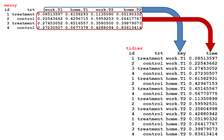
Let’s load the exper dataset. Have a look at it first. As you can see, the data format is wide. Each colunm has a location variable (home or office) for each treatment. What we will do is to convert the data from wide format to a long format. So, we will have two variables specified in two columns. The first variable is the location and the second variable is the time which reports the time required to go to a hospital from that location.
This is visually represented in the following image:
 Excercise
Practice on your R Studio line by line
library(tidyr)
exper <- read.csv("http://bit.ly/2kGgwd5")
head(exper)

widetolong <- exper %>% gather(key = location, value = time, work.T1:home.T2)
head(widetolong)
After converting from wide to long data format, let’s reverse the process: convert from long to wide using spread() function.
library(tidyr)

exper <- read.csv("http://bit.ly/2kGgwd5")
widetolong <- exper %>%
              gather(key = location, value = time, work.T1:home.T2)

longtowide <- widetolong %>%
              spread(location, time)
longtowide
2.4.3 Separate and Unite
The exper$casecode variable actually consists of 3 individual parts. The first digit represents the household identifier number, the second digit represents the number of female children under 5, and the last digit represents the total number of children under 5. So, for example, “111” means there is only one female child under 5 years old in the first household.
If we decide we want to create a new column for each taxonomic division of the casecode, we can accomplish this with separate() and undo it with unite().
Look up the help guide for the commands ?seperate and ?unite to familiarise with attributes of the commands.
# create new variables for each taxonomic component
exper_sep <- separate(exper, casecode, into = c("household", "girls", "totalkid"), sep = c(1,2,3))
exper_sep

# recombine the columns with unite
exper_rec <- unite(exper_sep, col = casecode, household:totalkid, sep = '')
exper_rec
Well-done! You have just completed the R-practical for Session 2. Now, go back to the lecture platform to take your R-test!
