Chapter 5 Correlation and Regression
In this session, we will explore regression and correlation. Both investigate the relationship between variables. In regression analysis, we model the relationship between:
- An outcome variable, \(y\), also called a dependent variable; and
- An explanatory/predictor variable, \(x\), also called an independent variable or predictor
Another way to state this is using mathematical terminology: we will model the outcome variable \(y\) as a function of the explanatory/predictor variable \(x\). Why do we have two different labels, explanatory and predictor, for the variable \(x\)? That is because, roughly speaking, data modelling can be used for two purposes:
Modelling for prediction: You want to predict an outcome variable \(y\) based on the information contained in a set of predictor variables. You do not have to worry too much about understanding how all the variables relate and interact, but so long as you can make good predictions about \(y\), you’re fine. For example, if we know many individuals’ risk factors for lung cancer, such as smoking habits and age, can we predict whether or not they will develop lung cancer? Here we don’t need to distinguish the degree to which the different risk factors contribute to lung cancer, we only need to focus on whether or not they could be put together to make reliable predictions.
Modelling for explanation: You want to explicitly describe the relationship between an outcome variable \(y\) and a set of explanatory variables, determine the significance of any found relationships, and have measures summarising these. Continuing our example from above, we would now be interested in describing the individual effects of the different risk factors and quantifying the magnitude of these effects. One solution could be to design an intervention to reduce lung cancer cases in a population, such as targeting smokers of a specific age group with advertisements for smoking cessation programs.
Data modelling is used in a wide variety of fields, including statistical inference, causal inference, artificial intelligence, and machine learning. There are many techniques for data modelling, such as tree-based models, neural networks/deep learning, and more. However, we’ll focus on one particular technique: linear regression, which is one of the most commonly-used and easy to understand approaches to modelling. Linear regression involves:
- An outcome variable \(y\) that is numerical and continuous
- Explanatory variables \(x\) that are either numerical or categorical
Whereas there is always only one numerical outcome variable \(y\), we have choices on both the number and the type of explanatory variables \(x\) to use. While in a simple linear regression, there is only one explanatory variable, in multiple linear regression, there are more than one explanatory variable.
5.1 Multiple Regression
In this practical, we’re going to study three multiple regression scenarios, where we have:
- Two explanatory variables \(x_1\) and \(x_2\) that are numerical and continuous,
- Two explanatory variables \(x_1\) (numerical) and \(x_2\) (categorical); and
- Three explanatory variables \(x_1\) (numerical), \(x_2\) (categorical) and \(x_3\) (interaction term).
We’ll study these regression scenarios using the dataset called credit, where predictions are made on the balance held by various credit card holders based on information like income, credit limit, and gender. Let’s consider the following variables:
- Outcome variable \(y\): Credit card balance in dollars
- Explanatory variables \(x\):
- Income in $1000’s
- Credit card limit in dollars
- Card holder’s age
- Gender.
Let’s load the packages we need for this session.
Before any regression analysis, we should explore the data first.
5.2 Exploratory Data Analysis
Firs thing first, let’s load the data and have a glimpse of it.
credit <- read_csv("http://bit.ly/33a5A8P")
glimpse(credit)
## Rows: 400
## Columns: 13
## $ ...1 <dbl> 1, 2, 3, 4, 5, 6, 7, 8, 9, 10, 11, 12, 13, 14~
## $ ID <dbl> 1, 2, 3, 4, 5, 6, 7, 8, 9, 10, 11, 12, 13, 14~
## $ Income <dbl> 14.891, 106.025, 104.593, 148.924, 55.882, 80~
## $ Limit <dbl> 3606, 6645, 7075, 9504, 4897, 8047, 3388, 711~
## $ Rating <dbl> 283, 483, 514, 681, 357, 569, 259, 512, 266, ~
## $ Cards <dbl> 2, 3, 4, 3, 2, 4, 2, 2, 5, 3, 4, 3, 1, 1, 2, ~
## $ Age <dbl> 34, 82, 71, 36, 68, 77, 37, 87, 66, 41, 30, 6~
## $ Education <dbl> 11, 15, 11, 11, 16, 10, 12, 9, 13, 19, 14, 16~
## $ Gender <chr> "Male", "Female", "Male", "Female", "Male", "~
## $ Student <chr> "No", "Yes", "No", "No", "No", "No", "No", "N~
## $ Married <chr> "Yes", "Yes", "No", "No", "Yes", "No", "No", ~
## $ Ethnicity <chr> "Caucasian", "Asian", "Asian", "Asian", "Cauc~
## $ Balance <dbl> 333, 903, 580, 964, 331, 1151, 203, 872, 279,~As you can see there are 13 variables and 400 observations in this dataset. However, we are interested in only the six variables listed above. So, we can select only these variables from the large dataset and create another one using the select() function of the dplyr package. We need to ensure that we have it installed and loaded first.
We should then have a quick look at the data again and produce summary statistics before running any models.
# Select the identified variables from the original large dataset:
credit_brief <- credit  %>%
  select(Balance, Limit, Income, Age, Gender)


# Summarise the dataset
summary(credit_brief)
## Balance Limit Income
## Min. : 0.00 Min. : 855 Min. : 10.35
## 1st Qu.: 68.75 1st Qu.: 3088 1st Qu.: 21.01
## Median : 459.50 Median : 4622 Median : 33.12
## Mean : 520.01 Mean : 4736 Mean : 45.22
## 3rd Qu.: 863.00 3rd Qu.: 5873 3rd Qu.: 57.47
## Max. :1999.00 Max. :13913 Max. :186.63
## Age Gender
## Min. :23.00 Length:400
## 1st Qu.:41.75 Class :character
## Median :56.00 Mode :character
## Mean :55.67
## 3rd Qu.:70.00
## Max. :98.00# Create a table of the variable Gender
table(credit_brief$Gender)##
## Female Male
## 207 193So, what do these summary statistics tell us? According to the summary statistics, we observe that:
- There are no missing values in our variables of interest;
- The average credit card balance is around $520;
- The average credit card limit is around $4800;
- The average income is around $45,200;
- There is almost an equal number of females and males in the data; and
- The average age is around 56.
On your own R Studio, keep going exploring these variables of interest. What is their standard deviation? How do their distributions look like?
Since our outcome variable Balance and the explanatory variables, Limit , Income and Age are numerical, we can compute the correlation coefficient between pairs of these variables. However, instead of running the cor() command for all pairwise comparison, we can simultaneously compute them by returning a correlation matrix below. We read off the correlation coefficient for any pair of variables by looking them up in the appropriate row/column combination.
credit %>%
  select(Balance, Limit, Income, Age) %>%
  cor()
## Balance Limit Income Age
## Balance 1.000000000 0.8616973 0.4636565 0.001835119
## Limit 0.861697267 1.0000000 0.7920883 0.100887922
## Income 0.463656457 0.7920883 1.0000000 0.175338403
## Age 0.001835119 0.1008879 0.1753384 1.000000000If you want to have a neater table, you can run the following which includes the knitr package and kable function. Note, this is optional. I am just demonstrating how you can get a nice-looking output here.
credit %>%
  select(Balance, Limit, Income, Age) %>%
  cor() %>%
  knitr::kable(
    digits = 3,
    caption = "Correlations between credit card balance, credit limit, credit rating, income and age",
    booktabs = TRUE
)| Balance | Limit | Income | Age | |
|---|---|---|---|---|
| Balance | 1.000 | 0.862 | 0.464 | 0.002 |
| Limit | 0.862 | 1.000 | 0.792 | 0.101 |
| Income | 0.464 | 0.792 | 1.000 | 0.175 |
| Age | 0.002 | 0.101 | 0.175 | 1.000 |
So, what does this correlation matrix tell us?
BalancewithLimitis 0.862, indicating a strong positive linear association;BalancewithIncomeis 0.464, suggestive of another positive linear association, although not as strong as the relationship betweenBalanceandLimit; and- The correlation coefficient between
LimitandIncomeis 0.792, indicating another strong association. - At the same time there is no correlation between
BalanceandAge.
Needless to say that any variable paired to itself (Balance-Balance, Limit-Limit, and so on) will have a correlation coefficient of 1.
Let’s visualise the association between the outcome variable with limit, income and age.
p1 <- ggplot(credit, aes(x = Age, y = Balance)) +
  geom_point() +
  labs(x = "Age", y = "Credit card balance (in $)", title = "Relationship between balance and age") +
  geom_smooth(method = "lm", se = FALSE)

p2 <- ggplot(credit, aes(x = Income, y = Balance)) +
  geom_point() +
  labs(x = "Income (in $1000)", y = "Credit card balance (in $)", title = "Relationship between balance and income") +
  geom_smooth(method = "lm", se = FALSE)

p3 <- ggplot(credit, aes(x = Limit, y = Balance)) +
  geom_point() +
  labs(x = "Limit", y = "Credit card balance (in $)", title = "Relationship between balance and limit") +
  geom_smooth(method = "lm", se = FALSE)

p1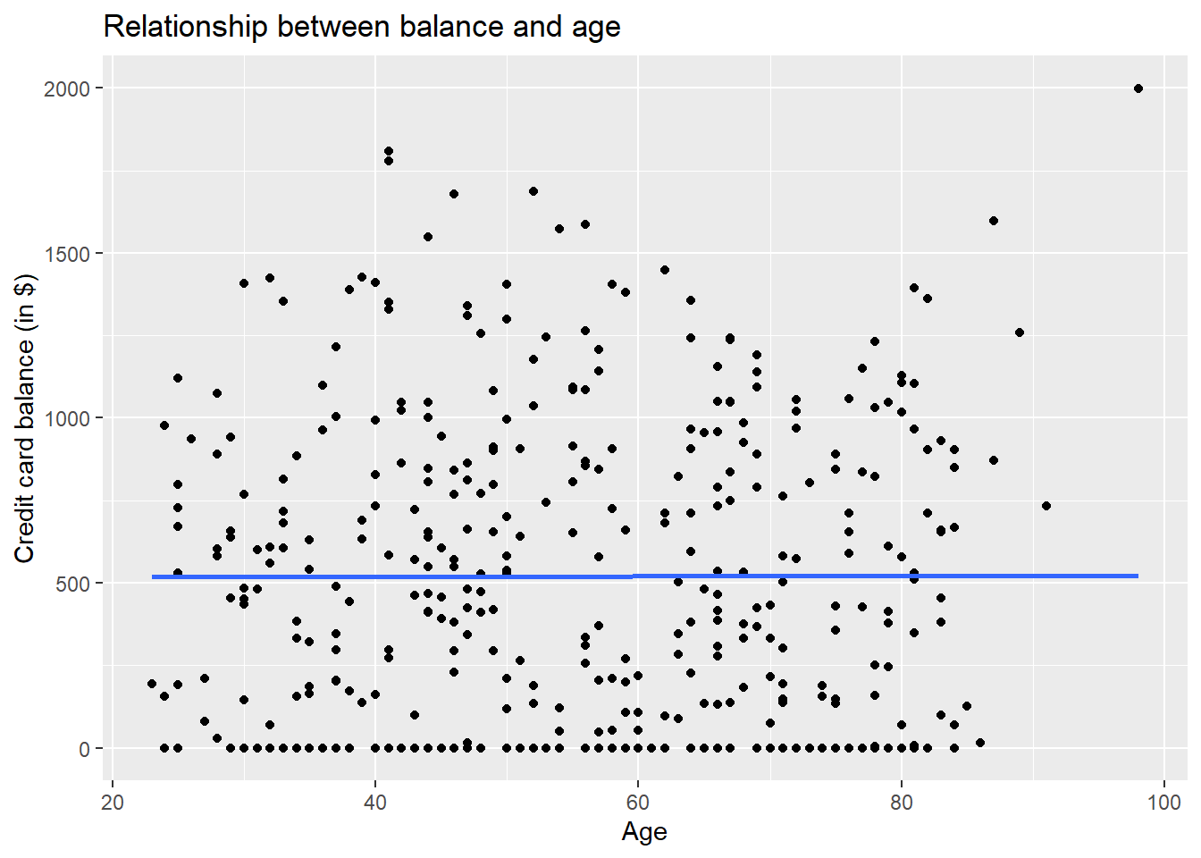
p2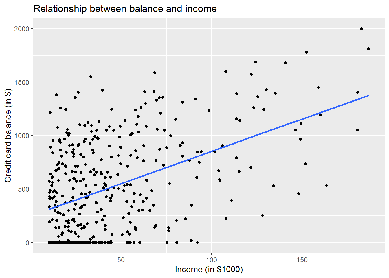
p3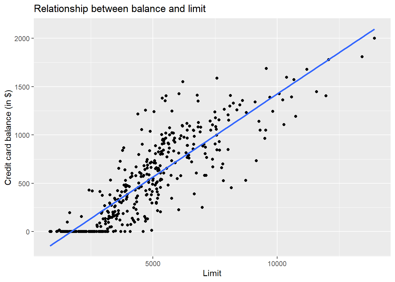
There seems to be a strong positive association between balance and two explanatory variables, namely limit and income, but weaker association with age.
5.3 Fitting Models
Let’s now try to identify factors that are associated with how much credit card debt an individual holds by setting up two multiple regression models described earlier.
5.3.1 Scenario 1: Numerical explanatory variables
We’ll perform multiple regression with:
- A numerical outcome variable \(y\), in this case credit card
Balance - Two explanatory variables:
- A first numerical explanatory variable \(x_1\), in this case
Age - A second numerical explanatory variable \(x_2\), in this case
Income
We run a regression using the lm function. We first indicate the dependent variable (i.e., Balance) and then explanatory variables (Balance ~ Income + Age), followed by the name of the data. To fit a regression model and obtain a summary of the results, you can use summary(). Let’s do this below:
credit <- read.csv("http://bit.ly/33a5A8P")
Balance_model <- lm(Balance ~ Income + Age, data = credit)
summary(Balance_model)
##
## Call:
## lm(formula = Balance ~ Income + Age, data = credit)
##
## Residuals:
## Min 1Q Median 3Q Max
## -864.15 -343.51 -51.42 317.95 1076.96
##
## Coefficients:
## Estimate Std. Error t value Pr(>|t|)
## (Intercept) 359.6727 70.3583 5.112 4.97e-07 ***
## Income 6.2359 0.5868 10.628 < 2e-16 ***
## Age -2.1851 1.1988 -1.823 0.0691 .
## ---
## Signif. codes: 0 '***' 0.001 '**' 0.01 '*' 0.05 '.' 0.1 ' ' 1
##
## Residual standard error: 406.7 on 397 degrees of freedom
## Multiple R-squared: 0.2215, Adjusted R-squared: 0.2176
## F-statistic: 56.47 on 2 and 397 DF, p-value: < 2.2e-16So, how do we interpret these three values presented in the regression output?
Intercept: 359.67. It is the predicted value of the dependent variable when all explanatory variables take a value of zero. In our case, when
incomeis zero and when age iszero. The intercept is used to situate the regression plane in 3D space.Income: 6.24. Now that we have multiple variables to consider, we have to add an important statement to our interpretation: all other things being equal, for every unit increase in annual income (which is measured in $1000’s), there is an associated increase of, on average, $6.24 in monthly credit card balance. So, this also says that every 84 pounds (1000/12) increase in monthly income would lead to around $7 increase in credit card balance, all else being constant.
Note:
* We are not making any causal statements here, only statements relating to the association between income and balance
* The all other things being equal statement addresses all other explanatory variables, in this case only one: Age. This is equivalent to saying “holding Age constant, we observed an associated increase of 6.24 dollar in credit card balance for every 1000 dollar increase in annual income.”
- Age: -2.18. Similarly, all other things being equal, when someone gets a year older, there is an associated decrease of on average $2.18 dollars in credit card balance.
5.3.2 Prediction
Suppose we want to use the model we created earlier to predict the credit card debt of a 35 years old individual who has an income of $30,000. If we wanted to do this by hand, we would simply plug in these values into the linear model:
\[ \begin{aligned} \widehat{y} &= b_0 + b_1 x_1 + b_2 x_2 \\ \widehat{credit} &= \hat{\beta}_0 + \hat{\beta}_1 income + \hat{\beta}_2 age \\ \end{aligned} \]
We can also calculate the predicted value in R.
First, we need to create a new dataframe for this individual:
newpers <- data.frame(Income = 30, Age = 35)
newpers
## Income Age
## 1 30 35Then, I can do the prediction using the predict function, after running the regression:
credit <- read.csv("http://bit.ly/33a5A8P")
newpers <- data.frame(Income = 30, Age = 35)
Balance_model <- lm(Balance ~ Income + Age, data = credit)
predict(Balance_model, newpers)
## 1
## 470.2718Here, using the model estimates from Balance_model, we find the predicted value of balance for newpers. So, the predicted credit card balance of a 35-years-old individual with an annual income of $30,000 is around $470. We can also construct a prediction interval around this prediction, which will provide a measure of uncertainty around the prediction. Remember, this is due to the error term we have in regression, which has zero mean and constant variance, and is independent of explanatory variables, \(x\).
newpers <- data.frame(Income = 30, Age = 35)
Balance_model <- lm(Balance ~ Income + Age, data = credit)
predict(Balance_model, newpers, interval = "prediction", level = 0.95)
## fit lwr upr
## 1 470.2718 -331.7286 1272.272Hence, the model predicts, with 95% confidence, that a 35-years-old person with an income of $30,000 is expected to have a credit card debt between approximately -$331 (negative sign indicates no debt) and $1272.
5.3.3 Scenario 2: Numerical and categorical explanatory variables
Let’s perform a multiple linear regression where we have a categorical and a continuous variable. Using the same data in Scenario 1, we have:
- A numerical outcome variable, \(y\), which is the credit card
Balance; - Three explanatory variables:
- A numerical \(x_1\), in this case
Income; - A numerical \(x_2\), in this case
age; and - A categorical variable, \(x_3\), in this case
gender.
Let’s visualise the relationship of the outcome variable with explanatory variables and see how this varies by gender.
p1 <- ggplot(credit, aes(x = Income, y = Balance, col = Gender)) +
  geom_point() +
  labs(x = "Income (in $1,000)", y = "Credit card balance (in $)", colour = "Gender") +
  geom_smooth(method = "lm", se = FALSE)

p2 <- ggplot(credit, aes(x = Age, y = Balance, col = Gender)) +
  geom_point() +
  labs(x = "Age", y = "Credit card balance (in $)", colour = "Gender") +
  geom_smooth(method = "lm", se = FALSE)

p1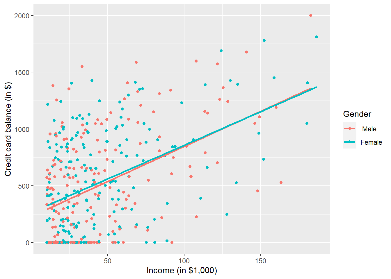
Figure 5.1: Instructor evaluation scores at UT Austin by gender
p2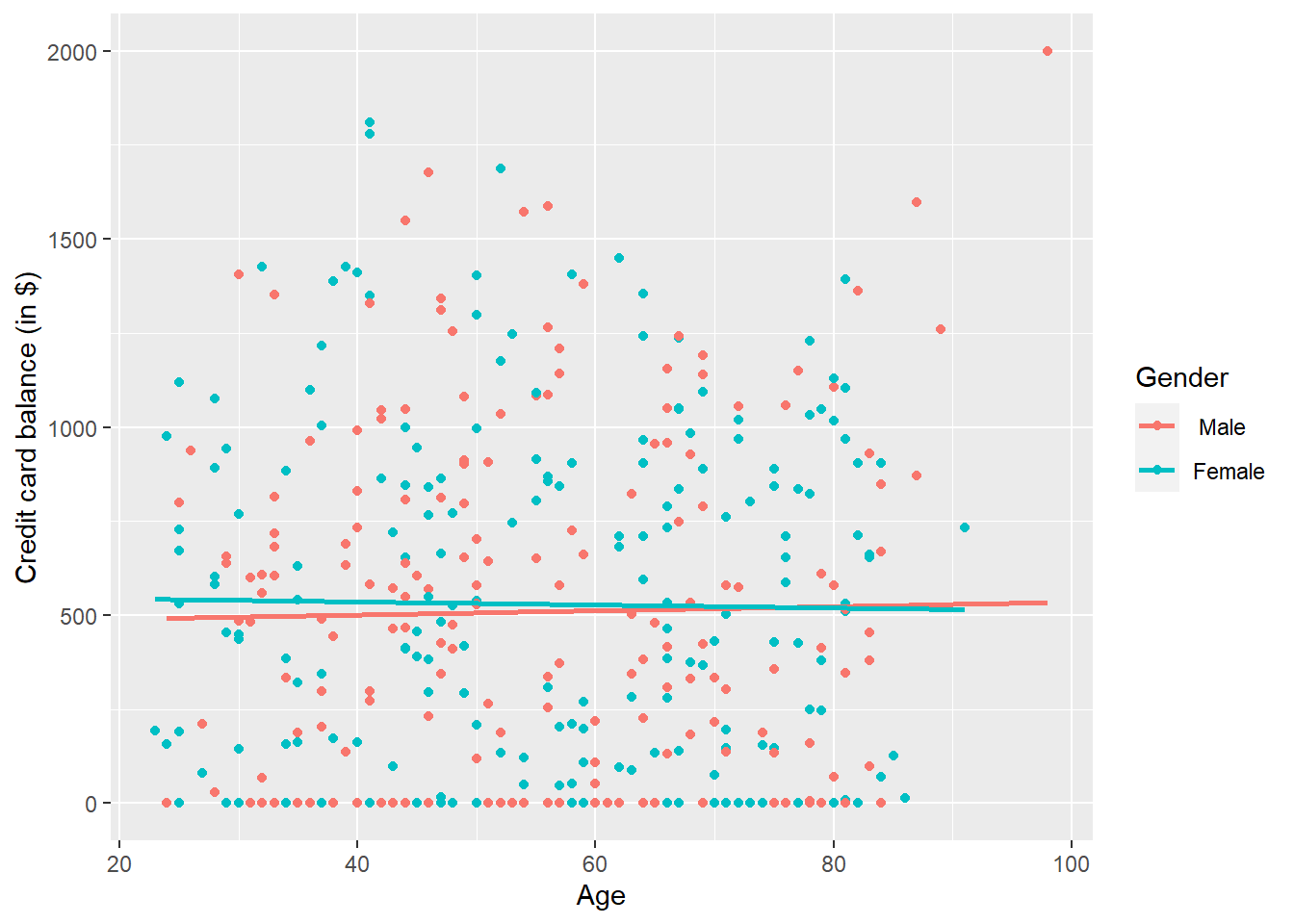
Figure 5.2: Instructor evaluation scores at UT Austin by gender
This is a scatterplot of Balance over Income and Age, but given that Gender is a binary categorical variable:
- We can assign a colour to points from each of the two levels of
Gender: female and male - Furthermore, the
geom_smooth(method = "lm", se = FALSE)layer automatically fits a different regression line for each gender category reported in the dataset.
We see that the associated effect of increasing age seems to be much harsher for women than men (at same age, women tend to have higher credit card balance than men). In other words, the regression lines for men and women have different slopes. Let’s run the regression to see if this difference is significant.
Balance_model2 <- lm(Balance ~ Income + Age + Gender, data = credit)
summary(Balance_model2)
##
## Call:
## lm(formula = Balance ~ Income + Age + Gender, data = credit)
##
## Residuals:
## Min 1Q Median 3Q Max
## -851.64 -339.21 -51.81 323.14 1089.77
##
## Coefficients:
## Estimate Std. Error t value Pr(>|t|)
## (Intercept) 346.9171 73.4748 4.722 3.25e-06 ***
## Income 6.2400 0.5873 10.626 < 2e-16 ***
## Age -2.1894 1.1998 -1.825 0.0688 .
## GenderFemale 24.7561 40.7284 0.608 0.5436
## ---
## Signif. codes: 0 '***' 0.001 '**' 0.01 '*' 0.05 '.' 0.1 ' ' 1
##
## Residual standard error: 407 on 396 degrees of freedom
## Multiple R-squared: 0.2222, Adjusted R-squared: 0.2163
## F-statistic: 37.71 on 3 and 396 DF, p-value: < 2.2e-16The modelling equation for this is: \[ \begin{aligned} \widehat{y} &= b_0 + b_1 x_1 + b_2 x_2 + b_3 x_3 \\ \widehat{credit} &= \hat{\beta}_0 + \hat{\beta}_1 income + \hat{\beta}_2 age + \hat{\beta}_3 female \\ \end{aligned} \]
We see that:
Males are treated as the baseline for comparison. The \(\beta_{female} = 24.75\) is the average difference in credit card balance that women get relative to the baseline of men. As you see from very high p-value, this coefficient is not significant - i.e., gender has no significant effect on credit card balance.
Accordingly, the intercepts are (although there is no practical interpretation of the intercept here, as discussed in Scenario 1):
- For men: \(\beta_0\) = -346.92
- For women: \(\beta_0 + \beta_{Female}\) = -346.92 + 24.75 = -322.17
Both men and women have the same slope for
incomeandage. In other words, in this model the associated effects of income and age are the same for men and women.
5.3.4 Prediction
Let’s predict the credit card debt of a 25-years-old female who has an annual income of $25,000.
\[ \begin{aligned} \widehat{y} &= b_0 + b_1 x_1 + b_2 x_2 + b_3 x_3 \\ \widehat{credit} &= \hat{\beta}_0 + \hat{\beta}_1 income + \hat{\beta}_2 age + \hat{\beta}_3 female \\ \end{aligned} \]
Let’s calculate the predicted value in R (remember, you just need to plug the values into the formula).
First, we need to create a new dataframe for this individual:
newpers2 <- data.frame(Income = 25, Age = 25, Gender = "Female")
newpers2
## Income Age Gender
## 1 25 25 FemaleThen, we can do the prediction using the predict function, after running the regression:
newpers2 <- data.frame(Income = 25, Age = 25, Gender = "Female")
Balance_model2 <- lm(Balance ~ Income + Age + Gender, data = credit)
predict(Balance_model2, newpers2)
## 1
## 472.938So, the predicted credit card balance for this individual is $472.94. We can also construct a prediction interval around this prediction as we did before. This will provide a measure of uncertainty around the prediction.
newpers2 <- data.frame(Income = 25, Age = 25, Gender = "Female")
Balance_model2 <- lm(Balance ~ Income + Age + Gender, data = credit)
predict(Balance_model2, newpers2, interval = "prediction", level = 0.95)
## fit lwr upr
## 1 472.938 -332.384 1278.26Hence, the model predicts, with 95% confidence, that a 25 years old female with an annual income of $25,000 is expected to have a credit card balance between approximately -$332 and $1,278.
If you were to find predicted the credit card balance for males, just type "Gender = " Male" where you specify the data frame for this new person above.
5.3.5 Scenario 3: Interaction Model
We say a model has an interaction effect if the associated effect of one variable depends on the value of another variable. Let’s now fit a model where we want to investigate whether there is a gender pay gap.
Balance_model3 <- lm(Balance ~ Income * Gender + Age, data = credit)
summary(Balance_model3)
##
## Call:
## lm(formula = Balance ~ Income * Gender + Age, data = credit)
##
## Residuals:
## Min 1Q Median 3Q Max
## -864.24 -341.81 -49.64 325.29 1092.19
##
## Coefficients:
## Estimate Std. Error t value Pr(>|t|)
## (Intercept) 338.4596 76.4074 4.430 1.22e-05 ***
## Income 6.4858 0.8410 7.712 1.02e-13 ***
## GenderFemale 46.2809 66.6002 0.695 0.4875
## Age -2.2390 1.2072 -1.855 0.0644 .
## Income:GenderFemale -0.4756 1.1636 -0.409 0.6830
## ---
## Signif. codes: 0 '***' 0.001 '**' 0.01 '*' 0.05 '.' 0.1 ' ' 1
##
## Residual standard error: 407.4 on 395 degrees of freedom
## Multiple R-squared: 0.2225, Adjusted R-squared: 0.2147
## F-statistic: 28.27 on 4 and 395 DF, p-value: < 2.2e-16The modelling equation for this is: \[ \begin{aligned} \widehat{y} &= b_0 + b_1 x_1 + b_2 x_2 + b_3 x_3 + b_4 x_2x_3\\ \widehat{credit} &= \hat{\beta}_0 + \hat{\beta}_1 income + \hat{\beta}_2 age + \hat{\beta}_3 female + \hat{\beta}_3 income female \\ \end{aligned} \]
We see that:
- Although not significant, the associated effect of income for women is less than males (i.e., interaction term). All other things being equal, for every 1,000 dollars increase in income, there is on average an associated decrease of \(\beta_{IncomeFemale}\) = -0.48 in credit card balance for women, as compared to men.
5.3.6 Prediction
Let’s recalculate the predicted value of credit card debt for the person we mentioned in Scenario 2, but now let’s take into account the interaction term.
We can also construct a prediction interval around this prediction, which will provide a measure of uncertainty around the prediction.
newpers2 <- data.frame(Income = 25, Age = 25, Gender = "Female")
Balance_model3 <- lm(Balance ~ Age +  Income * Gender, data = credit)
predict(Balance_model3, newpers2, interval = "prediction", level = 0.95)
## fit lwr upr
## 1 479.0224 -327.6851 1285.73The predicted value of credit card debt at 95% confidence level for a female participant with an income of $25,000 is expected to be between approximately $-328 and $1,286. As you see, this is not much different from the values obtained from the Scenario 2. This is mainly due to the insignificant interaction effect we had in Scenario 3.
5.4 Regression Conditions
Now, we know how to perform a regression analysis. However, the key question still remains: can we actually perform regression analysis? Do we comply with conditions that allow us to perform a regression analysis?
Let’s recap the regression conditions we have studied in the lecture:
- Linearity between the continuous (or numeric) dependent and continuous explanatory variables. Note that both variables need to be continuous as it does not make sense to have a linear relationship between a continuous dependent variable and a categorical explanatory variable;
- Having nearly normally distributed error terms;
- Constant variance of the error; and
- Independence of the observations in the data, and thus errors.
Let’s check these conditions using the same dataset above.
Linearity We will generate the residuals plot to test this. In multiple regression, the residual plot accommodates for other variables in the model, to see the trend in the relationship between the dependent and explanatory variables. Remember, in a simple linear regression where we have only one explanatory variable, a scatter plot would have been sufficient.
Let’s test the regression conditions for a regression, where we had income and age as explanatory variables and the balance as the dependent variable.
# Regression
Balance_model <- lm(Balance ~ Income + Age, data = credit)
# Residual plots
plot(Balance_model$residuals ~ credit$Age)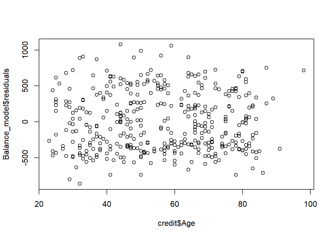
plot(Balance_model$residuals ~ credit$Income)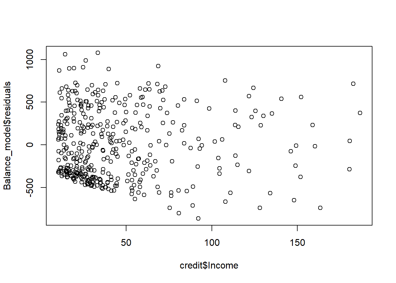
Remember, what we are looking for is a random scatter around zero. It seems like we are more or less meeting this condition for both variables, perhaps better for the age For variables that are not normal, we typically transform the data. For example, for variables like income, we take the logarithm of the variables so that the distribution of the transformed data pushes the data closer to a normal distribution.
# Transform income variable
log_transform <- credit %>% mutate(logincome = log(Income))
# Run regression using the log(income)
Balance_model_log <- lm(Balance ~ logincome + Age, data = log_transform)
# Residual plot for log(income)
plot(Balance_model_log$residuals ~ log_transform$logincome)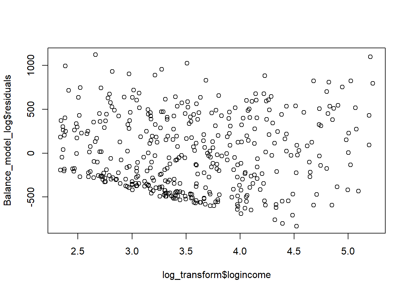 It seems like the log-transformation scattered the data points around the zero a little bit more. So, let’s use the logincome in our regression for the tests below as well.
Near normal residuals
We can investigate the normality of the residuals via a normal probability plot (QQ-plot).
log_transform <- credit %>% mutate(logincome = log(Income))
# Run regression using the log(income)
Balance_model_log <- lm(Balance ~ logincome + Age, data = log_transform)

hist(Balance_model_log$residuals)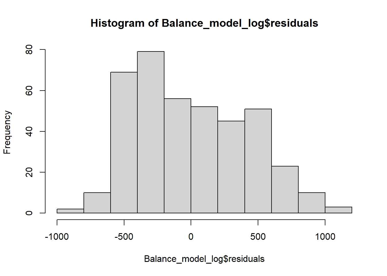
qqnorm(Balance_model_log$residuals)
qqline(Balance_model_log$residuals)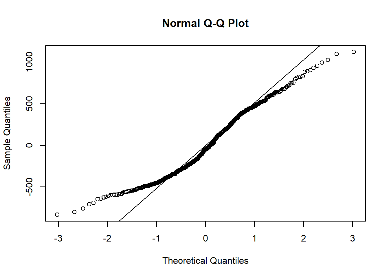

Figure 5.3: Designed by Allison Horst
We see a little bit of a right skew in the histogram and some data points are not on the straight line, especially those at the lower and upper tails, but otherwise we are not seeing massive deviations from the mean. So, we can say that this condition is somehow satisfied. Note that if you did not take the logarithm of the income and run the regression and test this, you would have similar results for this dataset.
Constant variability of residuals (or homoskedasticity) We basically want our residuals to have same variability for lower and higher values of the predicted outcome variable. So, we need to check the plot of residuals (e) versus the predicted y-hat (in this case, predicted credit card balance). Note that this is not the plot of residuals versus x, but takes into account all explanatory variables in the model at once by finding the predicted y-hat. What we expect from this plot is randomly scattered residuals around zero without any obvious pattern, like a fan-shape.
# Transform income variable
log_transform <- credit %>% mutate(logincome = log(Income))
# Run regression using the log(income)
Balance_model_log <- lm(Balance ~ logincome + Age, data = log_transform)
plot(Balance_model_log$residuals ~ Balance_model_log$fitted)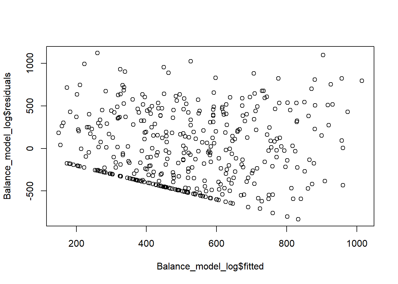 We have residuals on y-axis, and fitted-values (y-hat) on the x-axis. Constant variance assumption does not seem to be satisfied as we see a pattern where residuals do not seem to be contained in a constant distance from the mean.
Independent residuals
This means that observations are independent from each other, rather than having a time-series structure. So, we look at the plot of residuals and see whether there is anything strange happening, such as a pattern, in the order the data points in our dataset. Once we plot the residuals again using plot(Balance_model_log$residuals), we see no increasing or decreasing pattern, so it appears to be residuals are independent from each other.
Figure 5.4: Designed by Seda Erdem
This work uses materials that are licensed under Creative Commons Attribution-ShareAlike 3.0 Unported. It includes materials that are designed by OpenIntro.