Chapter 7 Logistic Regression

Logistic regression is the standard way to model binary outcomes- that is, data $y_i$ that take on the values 0 or 1.

• When we have an binary outcome $Y$, the process can be considered as a Bernoulli trial with the success probability $\pi$.
• Like linear regression for a continuous outcome, we’re modelling $E(Y)$ in connection with predictors, $E(Y)\sim X$.
• We know that $E(Y)=\pi$.
• The regression form can be $$\pi = P(Y_i=1) = f(x)$$
• Here, the probability $\pi$ should be in $[0,1]$, however $x$ can be in any range.
• So the function $f(\cdot)$ should be $f: R \mapsto (0,1)$
• The logistic regression uses the logistic function on the linear combination of predictors: $$\pi_i= P(y_i=1) = \frac{\exp(X_i\beta)}{1+\exp(X_i\beta)}$$

logistic_f <- function(x){1/(1+exp(-x))}
x = seq(-10,10,by=0.1)
plot(x,logistic_f(x),type='l',xlab=expression(paste(X,beta)),ylab='logistic_f')
abline(h=0.5,lty=2,col=3)
abline(v=0,lty=2,col=3)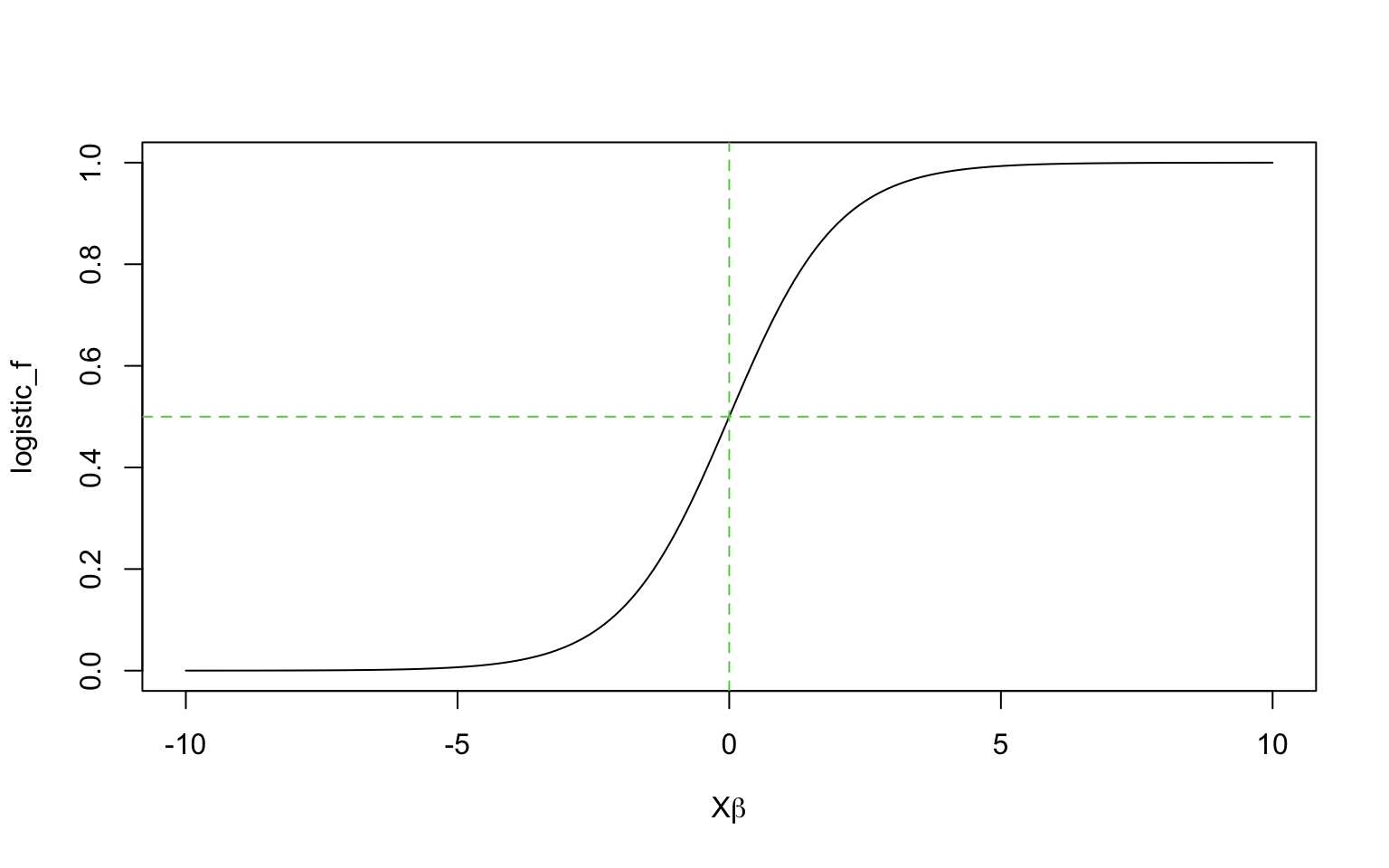

• As seen from the above, the logistic function is curved, the expected difference in $Y$ corresponding to a fixed difference in $X$ is not a constant.

  • The steepest change occurs at the middle of the curve
  • When the change in probability is compressed at the ends, which is needed to keep probabilies bounded between 0 and 1.

• In statistics, it is more interpretable when we reexpress it: $$\log(\frac{\pi_i}{1-\pi_i}) = logit(\pi_i) = X_i\beta,$$ where the inverse of $logit$ is the logistic function.

• From the perspective of a generalized linear model (GLM), the linear combination of predictors is linked to the mean of the outcome variable through the $logit$ link function.

• The $logit(\pi_i)$ can be interpreted as $log(Odds_i)$.

7.1 Single predictor

7.1.1 Example : modeling political preference given income

Conservative parties generally receive more support among voters with high incomes. We illustrate classical logistic regression with a simple analysis of this pattern from the National Election Study in 1992. For each respondent $i$ in this poll, we label $y_i=1$ if he or she preferred George Bush (the Republican) or 0 if Bill Clinton (the Democratic), excluding respondents who preferred other candidates or had no opinion.

library(tidyverse)
load("files/GelmanData/USA1992election.rda")
attach(data)
yr <- 1992
ok <- presvote<3
vote <- presvote[ok] - 1 # 1 for Geourge, 0 for Clinton
income <- data$income[ok] # 1=poor to 5=rich
ta = table(vote,income)
ta

##     income
## vote    1    2    3    4    5
##    0  980 1186 2191 2032  268
##    1  701  978 2222 2540  659

prop.table(ta, margin=2) # you can check it increasing

##     income
## vote         1         2         3         4         5
##    0 0.5829863 0.5480591 0.4964877 0.4444444 0.2891046
##    1 0.4170137 0.4519409 0.5035123 0.5555556 0.7108954

# Visualization first
df = data.frame(income=income,vote=vote)
ggplot(df, aes(x = income, y = vote)) +
  geom_point(alpha = 0.05, position = position_jitter(height = 0.02)) +
  geom_smooth(method = "glm", method.args = list(family = "binomial"),
              se = TRUE, color = "red") +
  labs(title = "Logistic Fit",y='P(vote for republican)')+
  theme_classic()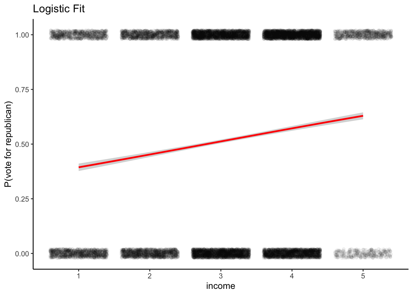

# Estimation
fit.1 <- glm (vote ~ income, family=binomial(link="logit"))
summary(fit.1)

## 
## Call:
## glm(formula = vote ~ income, family = binomial(link = "logit"))
## 
## Coefficients:
##             Estimate Std. Error z value Pr(>|z|)    
## (Intercept) -0.67108    0.05077  -13.22   <2e-16 ***
## income       0.24012    0.01559   15.40   <2e-16 ***
## ---
## Signif. codes:  0 '***' 0.001 '**' 0.01 '*' 0.05 '.' 0.1 ' ' 1
## 
## (Dispersion parameter for binomial family taken to be 1)
## 
##     Null deviance: 19057  on 13756  degrees of freedom
## Residual deviance: 18815  on 13755  degrees of freedom
##   (20877 observations deleted due to missingness)
## AIC: 18819
## 
## Number of Fisher Scoring iterations: 4

$\pi$, the probability of republican support is fitted : $$logit(\pi) = -0.67 + 0.24\cdot Income$$

Equivalently, we can express it: $$\pi = logit^{-1}(-0.67 + 0.24\cdot Income)$$

The above figure shows the fitting.

Interpretation:

• Intercept is not interesting

• A difference of 1 in income level corresponds to a positive difference of of 0.24 in logOdds (logit probability) of supporting republican.

• A unit difference in Income corresponds to a multiplicative change of $e^{0.24}=1.27$ in the odds

• Interpretation in predicted probability of supporting Bush.

  • What is the probability of republican support at the income level=3?
  • We can evaluate how the probability differs with a unit difference in $x$ near the central value, at $Income=3$ and $Income=2$, $P(y=1|Income=3) - P(y=1|Income=2)$.
  • How about between $Income=4$ and $Income=5$

logistic_f(-0.67+0.24*3)

## [1] 0.5124974

logistic_f(-0.67+0.24*3)-logistic_f(-0.67+0.24*2)

## [1] 0.05985501

logistic_f(-0.67+0.24*5)-logistic_f(-0.67+0.24*4)

## [1] 0.05748698

In the range of Income =1 to 5, the fitted line is almost linear (see plot above). We can interpret that a difference of 1 in income level corresponds to a positive difference of 6% in the probability of supporting the republican.

• Or, we can consider a small unit change by differentiating the logistic function w.r.t. $x$: $$\beta e^{\alpha+\beta x}/(1+e^{\alpha+\beta x})^2$$

• The derivative (slope) is maximized at the center, $\alpha+\beta x =0$, which gives the logistic function value of 0.5. If we plug this into the above, we get $\beta/4$.

• Thus, $\beta/4$ is the maximum difference is the maximum difference in $P(y=1)$ corresponding to a unit difference in $x$.

• As a rule of convenience, we can compute $\beta/4$ to get an upper bound of the predictive difference corresponding to a unit difference in $x$.

• In the example, $\beta/4=0.06$: a difference of 1 in income category corresponds to no more than an 6% positive difference in the probability of supporting Bush.

7.2 Building a logistic model

We learn the steps of building, understanding, and checking the fit of a logistic regression model using an exampling: modeling the decisions of households in Bangladesh about whether to change their source of drinking water.

library(tidyverse)
wells <- read.table ("files/GelmanData/wells.dat")
attach(wells)

Background:

• Many of the wells used for drinking water in Bangladesh and other South Asian countries are contaminated with natural arsenic, affecting an estimated 100 million people.

• Arsenic is a cumulative poison, and exposure increases the risk of cancer and other diseases, with risks estimated to be proportional to exposure.

• A research team from the United States and Bangladesh measured all the wells and labeled them with their arsenic level as well as characterization as ‘safe’ (below 0.5 in units of hundreds of micrograms per liter, the Bangladesh standard for arsenic in drinking water) or ‘unsafe’ (above 0.5).

• People with unsafe wells were encouraged to switch to nearby wells or to new wells of their own construction

• A few years later, the researchers returned to find out who had switched wells.

• We aim to understand the factors predictive of well switching among users of unsafe wells.

Outcome

• The outcome variable is $y_i=1$ if household $i$ switched to a new well, and 0 if household $i$ continued using its own well.

Input

• A constant term

• The distance (in meters) to the closest known safe well

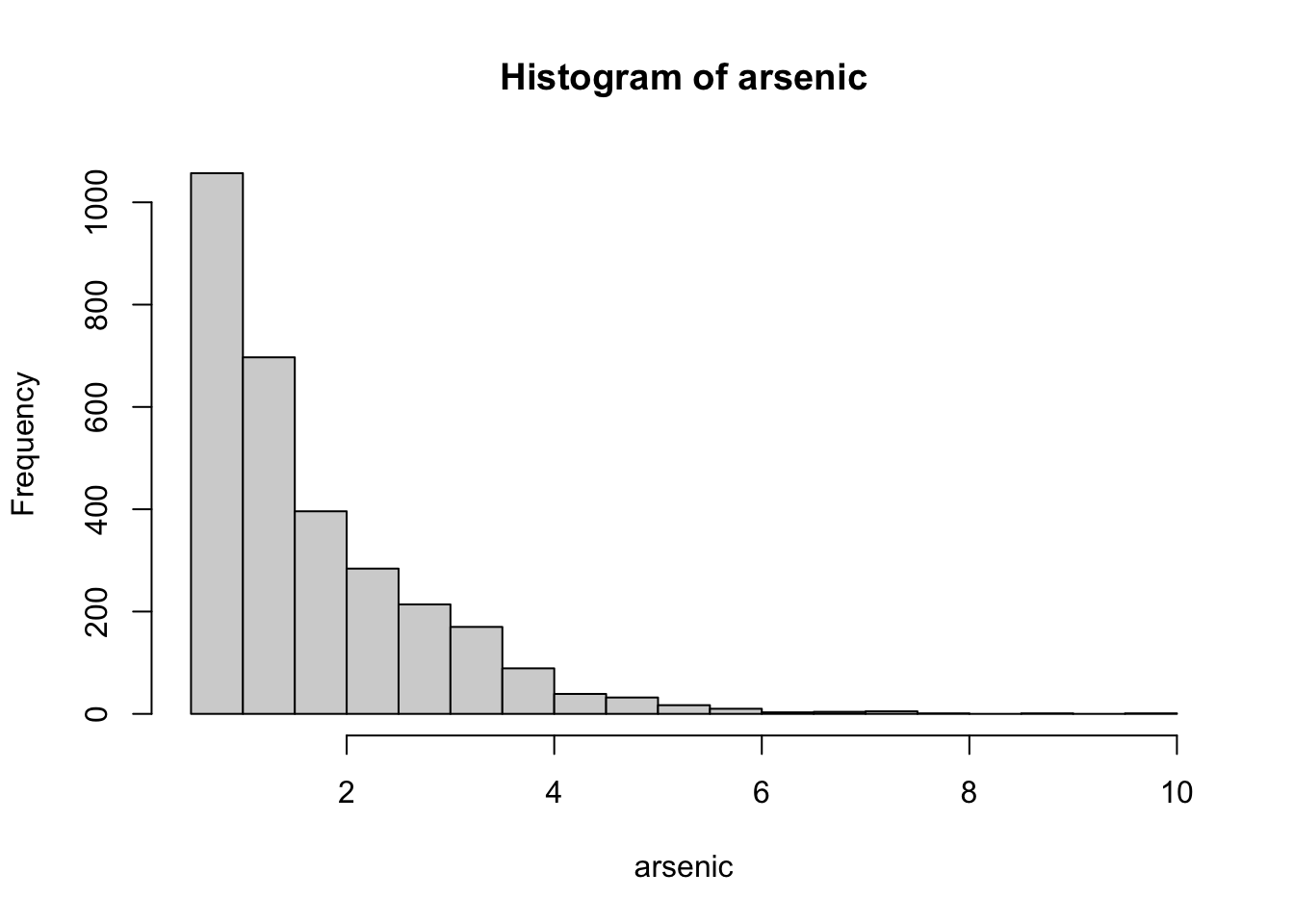
• The arsenic level of respondent’s well

• Whether any members of the household are active in community organizations

• The education level of the head of household

7.2.1 One predictor model

We first consider to use the distance variable.

fit1 <- glm (switch ~ dist, family=binomial(link='logit'))
summary(fit1)

## 
## Call:
## glm(formula = switch ~ dist, family = binomial(link = "logit"))
## 
## Coefficients:
##               Estimate Std. Error z value Pr(>|z|)    
## (Intercept)  0.6059594  0.0603102  10.047  < 2e-16 ***
## dist        -0.0062188  0.0009743  -6.383 1.74e-10 ***
## ---
## Signif. codes:  0 '***' 0.001 '**' 0.01 '*' 0.05 '.' 0.1 ' ' 1
## 
## (Dispersion parameter for binomial family taken to be 1)
## 
##     Null deviance: 4118.1  on 3019  degrees of freedom
## Residual deviance: 4076.2  on 3018  degrees of freedom
## AIC: 4080.2
## 
## Number of Fisher Scoring iterations: 4

• The coefficient for dist is -0.0062, which seems low, but this is misleading.

• Let’s change it into 100 meter unit. Then the coefficient becomes -0.62.

• We transform the unit of the predictor.

dat <- wells %>% mutate(dist100 = dist/100)
fit1 <- glm (switch ~ dist100, family=binomial(link='logit'),data=dat)
summary(fit1)

## 
## Call:
## glm(formula = switch ~ dist100, family = binomial(link = "logit"), 
##     data = dat)
## 
## Coefficients:
##             Estimate Std. Error z value Pr(>|z|)    
## (Intercept)  0.60596    0.06031  10.047  < 2e-16 ***
## dist100     -0.62188    0.09743  -6.383 1.74e-10 ***
## ---
## Signif. codes:  0 '***' 0.001 '**' 0.01 '*' 0.05 '.' 0.1 ' ' 1
## 
## (Dispersion parameter for binomial family taken to be 1)
## 
##     Null deviance: 4118.1  on 3019  degrees of freedom
## Residual deviance: 4076.2  on 3018  degrees of freedom
## AIC: 4080.2
## 
## Number of Fisher Scoring iterations: 4

Visualize the fitting

ggplot(dat, aes(x = dist100, y = switch)) +
  geom_point(alpha = 0.05, position = position_jitter(height = 0.02)) +
  geom_smooth(method = "glm", method.args = list(family = "binomial"),
              se = TRUE, color = "red") +
  labs(title = "Logistic Fit",y='P(Switch)', x='Distance (in 100 meters) to nearest safe well')+
  theme_classic()

## `geom_smooth()` using formula = 'y ~ x'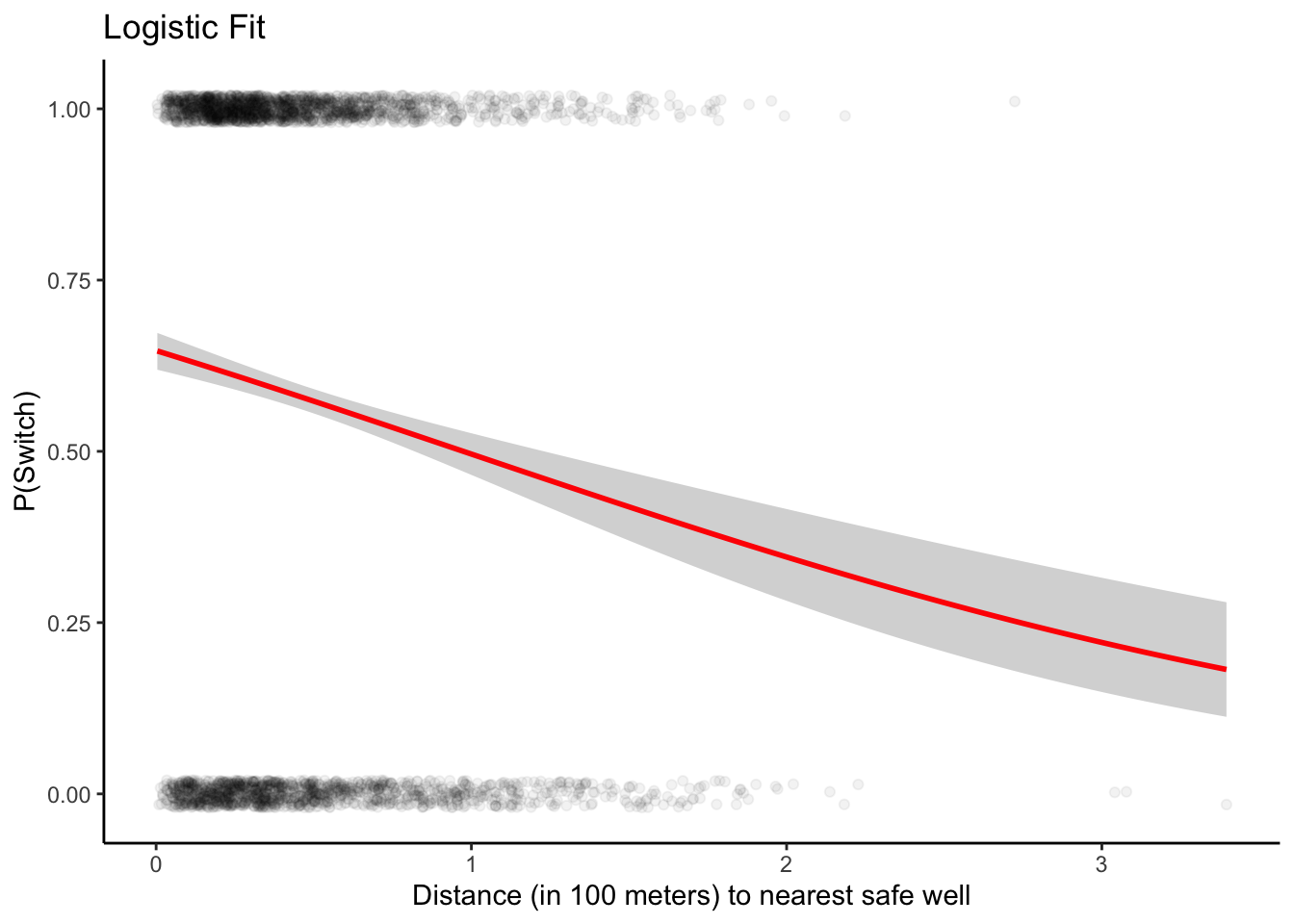

Interpretation of the fitting

• The probability of switching is about 60% for people who live near a safe well, declining to about 20% for people who live more than 300 meters from any safe well.

• Intercept: the probability of switching is $logit^{-1}(0.61)$ = 0.65. Thus, the model estimates a 65% probability of switching if you live right next to an existing safe well.

• The derivative at the average value in dist100: from the derivative $\beta e^{\alpha+\beta x}/(1+e^{\alpha+\beta x})^2$ So the slope of the curve at the average value is:

mm <- with(dat,mean(dist100))
# The value of linear function at mm
beta <- coef(fit1) 
lv <- beta[1] + beta[2]*mm
beta[2]*exp(lv) / (1+exp(lv))^2

##    dist100 
## -0.1519011

Thus, adding 100 meters to the distance to the nearest safe well- correponds to a decrease in the probability of switching of about 15%.

• The ‘divide by 4 rule’:

beta[2]/4

##    dist100 
## -0.1554705

This comes out similar as was calculated using the derivative because the curve passes through the 50% point.

7.2.2 Adding a second input variable

We now add arsenic level of the existing well.

hist(arsenic,breaks=30)

fit2 <- glm (switch ~ dist100 + arsenic, family=binomial(link='logit'),data=dat)
summary(fit2)

## 
## Call:
## glm(formula = switch ~ dist100 + arsenic, family = binomial(link = "logit"), 
##     data = dat)
## 
## Coefficients:
##              Estimate Std. Error z value Pr(>|z|)    
## (Intercept)  0.002749   0.079448   0.035    0.972    
## dist100     -0.896644   0.104347  -8.593   <2e-16 ***
## arsenic      0.460775   0.041385  11.134   <2e-16 ***
## ---
## Signif. codes:  0 '***' 0.001 '**' 0.01 '*' 0.05 '.' 0.1 ' ' 1
## 
## (Dispersion parameter for binomial family taken to be 1)
## 
##     Null deviance: 4118.1  on 3019  degrees of freedom
## Residual deviance: 3930.7  on 3017  degrees of freedom
## AIC: 3936.7
## 
## Number of Fisher Scoring iterations: 4

Both regression coefficients were significant: switching is easier if there is a nearby safe well, and if a household’s existing well has a high arsenic level. There should be more motivation to switch.

• The ‘divide by 4 rule’:

beta <- coef(fit2)
beta[2]/4

##   dist100 
## -0.224161

beta[3]/4

##   arsenic 
## 0.1151937

100 meters more in distance correponds to an approximately 22% lower probability of switching, and 1 unit more in arsenic concentration correponds to an approximately 11% positive difference in switching probability.

Effect of arsenic level adjustment for the relation of switching ~ dist: The coefficient for dist100 changes from -0.62 to -0.90 after adjustment of arsenic level.

We can visualize the fitted lines.

arsenic_seq <- seq(min(dat$arsenic), max(dat$arsenic), length.out = 100)

# Prediction when dist100 = mean
df_mean <- data.frame(
  arsenic = arsenic_seq,
  dist100 = mean(dat$dist100)
) %>%
  mutate(pred = predict(fit2, newdata = ., type = "response"),
         label = "dist100 = mean")

# Prediction when dist100 = 0
df_zero <- data.frame(
  arsenic = arsenic_seq,
  dist100 = 0
) %>%
  mutate(pred = predict(fit2, newdata = ., type = "response"),
         label = "dist100 = 0")

# Combine both
df_pred <- bind_rows(df_mean, df_zero)

# Plot raw data and prediction lines
ggplot(dat, aes(x = arsenic, y = switch)) +
  geom_jitter(height = 0.05, width = 0, alpha = 0.3) +
  geom_line(data = df_pred, aes(x = arsenic, y = pred, color = label), size = 1.2) +
  labs(
    title = "Predicted Probability of Switching",
    x = "Arsenic Level",
    y = "Probability",
    color = "dist100 value"
  ) +
  theme_minimal()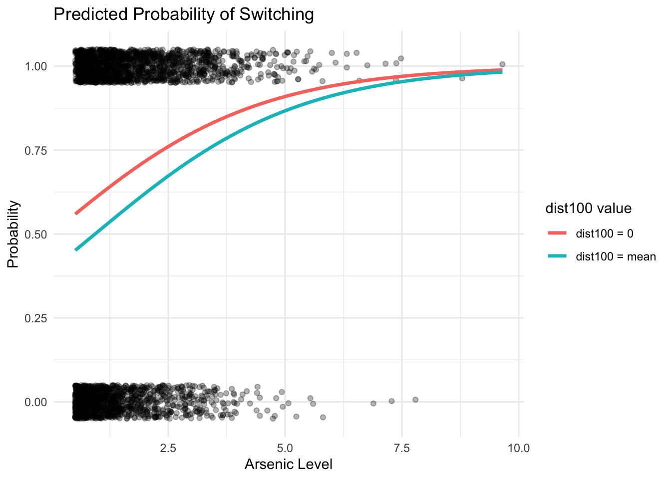

7.2.3 With interaction

fit3 <- glm (switch ~ dist100*arsenic, family=binomial(link='logit'),data=dat)
summary(fit3)

## 
## Call:
## glm(formula = switch ~ dist100 * arsenic, family = binomial(link = "logit"), 
##     data = dat)
## 
## Coefficients:
##                 Estimate Std. Error z value Pr(>|z|)    
## (Intercept)     -0.14787    0.11754  -1.258  0.20838    
## dist100         -0.57722    0.20918  -2.759  0.00579 ** 
## arsenic          0.55598    0.06932   8.021 1.05e-15 ***
## dist100:arsenic -0.17891    0.10233  -1.748  0.08040 .  
## ---
## Signif. codes:  0 '***' 0.001 '**' 0.01 '*' 0.05 '.' 0.1 ' ' 1
## 
## (Dispersion parameter for binomial family taken to be 1)
## 
##     Null deviance: 4118.1  on 3019  degrees of freedom
## Residual deviance: 3927.6  on 3016  degrees of freedom
## AIC: 3935.6
## 
## Number of Fisher Scoring iterations: 4

Interpretation of the coefficient for interaction term:

• for each additional unit of arsenic, the value -0.18 is added to the coefficient for distance
• for each additional unit of dist100, the value -0.18 is added to the coefficient for arsenic

# Prediction when dist100 = mean
df_mean <- data.frame(
  arsenic = arsenic_seq,
  dist100 = mean(dat$dist100)
) %>%
  mutate(pred = predict(fit3, newdata = ., type = "response"),
         label = "dist100 = mean")

# Prediction when dist100 = 0
df_zero <- data.frame(
  arsenic = arsenic_seq,
  dist100 = 0
) %>%
  mutate(pred = predict(fit3, newdata = ., type = "response"),
         label = "dist100 = 0")

# Combine both
df_pred <- bind_rows(df_mean, df_zero)

# Plot raw data and prediction lines
ggplot(dat, aes(x = arsenic, y = switch)) +
  geom_jitter(height = 0.05, width = 0, alpha = 0.3) +
  geom_line(data = df_pred, aes(x = arsenic, y = pred, color = label), size = 1.2) +
  labs(
    title = "Predicted Probability of Switching",
    x = "Arsenic Level",
    y = "Probability",
    color = "dist100 value"
  ) +
  theme_minimal()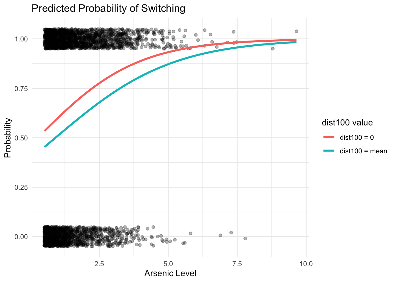

7.2.4 Additing social predictors

• assoc=1 if a household member is in any community organization
• educ = years of education of the well user

dat <- dat %>% mutate(educ4 = educ/4)
fit4 <- glm (switch ~ arsenic + dist100 + assoc + educ4, family=binomial(link='logit'),data=dat)
summary(fit4)

## 
## Call:
## glm(formula = switch ~ arsenic + dist100 + assoc + educ4, family = binomial(link = "logit"), 
##     data = dat)
## 
## Coefficients:
##             Estimate Std. Error z value Pr(>|z|)    
## (Intercept) -0.15671    0.09960  -1.573    0.116    
## arsenic      0.46702    0.04160  11.226  < 2e-16 ***
## dist100     -0.89611    0.10458  -8.569  < 2e-16 ***
## assoc       -0.12430    0.07697  -1.615    0.106    
## educ4        0.16979    0.03835   4.427 9.55e-06 ***
## ---
## Signif. codes:  0 '***' 0.001 '**' 0.01 '*' 0.05 '.' 0.1 ' ' 1
## 
## (Dispersion parameter for binomial family taken to be 1)
## 
##     Null deviance: 4118.1  on 3019  degrees of freedom
## Residual deviance: 3907.8  on 3015  degrees of freedom
## AIC: 3917.8
## 
## Number of Fisher Scoring iterations: 4

Let’s try the full model including all possible interactions:

fit.ful <- glm (switch ~ arsenic * dist100 * assoc * educ4, family=binomial,data=dat)
fit.null <- glm (switch ~ 1, family=binomial,data=dat)
summary(fit.ful)

## 
## Call:
## glm(formula = switch ~ arsenic * dist100 * assoc * educ4, family = binomial, 
##     data = dat)
## 
## Coefficients:
##                             Estimate Std. Error z value Pr(>|z|)    
## (Intercept)                 -0.16555    0.24605  -0.673  0.50105    
## arsenic                      0.61428    0.14482   4.242 2.22e-05 ***
## dist100                     -1.00933    0.43775  -2.306  0.02113 *  
## assoc                        0.73297    0.37606   1.949  0.05129 .  
## educ4                       -0.06943    0.15415  -0.450  0.65243    
## arsenic:dist100             -0.24618    0.20598  -1.195  0.23203    
## arsenic:assoc               -0.56435    0.21499  -2.625  0.00866 ** 
## dist100:assoc               -1.03348    0.71359  -1.448  0.14754    
## arsenic:educ4                0.07170    0.09345   0.767  0.44292    
## dist100:educ4                0.38868    0.28079   1.384  0.16628    
## assoc:educ4                 -0.39631    0.24695  -1.605  0.10853    
## arsenic:dist100:assoc        0.73230    0.33086   2.213  0.02687 *  
## arsenic:dist100:educ4       -0.01600    0.13854  -0.116  0.90804    
## arsenic:assoc:educ4          0.20829    0.14937   1.394  0.16319    
## dist100:assoc:educ4          0.60129    0.46414   1.295  0.19516    
## arsenic:dist100:assoc:educ4 -0.37745    0.23019  -1.640  0.10106    
## ---
## Signif. codes:  0 '***' 0.001 '**' 0.01 '*' 0.05 '.' 0.1 ' ' 1
## 
## (Dispersion parameter for binomial family taken to be 1)
## 
##     Null deviance: 4118.1  on 3019  degrees of freedom
## Residual deviance: 3876.0  on 3004  degrees of freedom
## AIC: 3908
## 
## Number of Fisher Scoring iterations: 4

fit = step(fit.null,scope = list(lower = fit.null, upper = fit.ful),
                    direction = "forward")

## Start:  AIC=4120.1
## switch ~ 1
## 
##           Df Deviance    AIC
## + arsenic  1   4008.7 4012.7
## + dist100  1   4076.2 4080.2
## + educ4    1   4100.4 4104.4
## + assoc    1   4114.2 4118.2
## <none>         4118.1 4120.1
## 
## Step:  AIC=4012.67
## switch ~ arsenic
## 
##           Df Deviance    AIC
## + dist100  1   3930.7 3936.7
## + educ4    1   3987.7 3993.7
## + assoc    1   4005.7 4011.7
## <none>         4008.7 4012.7
## 
## Step:  AIC=3936.67
## switch ~ arsenic + dist100
## 
##                   Df Deviance    AIC
## + educ4            1   3910.4 3918.4
## + arsenic:dist100  1   3927.6 3935.6
## + assoc            1   3927.7 3935.7
## <none>                 3930.7 3936.7
## 
## Step:  AIC=3918.43
## switch ~ arsenic + dist100 + educ4
## 
##                   Df Deviance    AIC
## + dist100:educ4    1   3896.2 3906.2
## + arsenic:educ4    1   3902.9 3912.9
## + assoc            1   3907.8 3917.8
## + arsenic:dist100  1   3907.9 3917.9
## <none>                 3910.4 3918.4
## 
## Step:  AIC=3906.15
## switch ~ arsenic + dist100 + educ4 + dist100:educ4
## 
##                   Df Deviance    AIC
## + arsenic:educ4    1   3893.0 3905.0
## + assoc            1   3893.1 3905.1
## <none>                 3896.2 3906.2
## + arsenic:dist100  1   3894.5 3906.5
## 
## Step:  AIC=3905.03
## switch ~ arsenic + dist100 + educ4 + dist100:educ4 + arsenic:educ4
## 
##                   Df Deviance    AIC
## + assoc            1   3890.1 3904.1
## <none>                 3893.0 3905.0
## + arsenic:dist100  1   3891.7 3905.7
## 
## Step:  AIC=3904.1
## switch ~ arsenic + dist100 + educ4 + assoc + dist100:educ4 + 
##     arsenic:educ4
## 
##                   Df Deviance    AIC
## + arsenic:assoc    1   3887.4 3903.4
## <none>                 3890.1 3904.1
## + assoc:educ4      1   3888.6 3904.6
## + arsenic:dist100  1   3888.9 3904.9
## + dist100:assoc    1   3889.8 3905.8
## 
## Step:  AIC=3903.41
## switch ~ arsenic + dist100 + educ4 + assoc + dist100:educ4 + 
##     arsenic:educ4 + arsenic:assoc
## 
##                   Df Deviance    AIC
## <none>                 3887.4 3903.4
## + assoc:educ4      1   3885.6 3903.6
## + arsenic:dist100  1   3886.3 3904.3
## + dist100:assoc    1   3886.4 3904.4

summary(fit)

## 
## Call:
## glm(formula = switch ~ arsenic + dist100 + educ4 + assoc + dist100:educ4 + 
##     arsenic:educ4 + arsenic:assoc, family = binomial, data = dat)
## 
## Coefficients:
##               Estimate Std. Error z value Pr(>|z|)    
## (Intercept)    0.06895    0.13881   0.497  0.61937    
## arsenic        0.45680    0.07248   6.302 2.93e-10 ***
## dist100       -1.32714    0.17510  -7.579 3.47e-14 ***
## educ4         -0.10092    0.07982  -1.264  0.20610    
## assoc          0.06878    0.14474   0.475  0.63465    
## dist100:educ4  0.33775    0.10672   3.165  0.00155 ** 
## arsenic:educ4  0.07446    0.04358   1.708  0.08756 .  
## arsenic:assoc -0.13240    0.08056  -1.644  0.10026    
## ---
## Signif. codes:  0 '***' 0.001 '**' 0.01 '*' 0.05 '.' 0.1 ' ' 1
## 
## (Dispersion parameter for binomial family taken to be 1)
## 
##     Null deviance: 4118.1  on 3019  degrees of freedom
## Residual deviance: 3887.4  on 3012  degrees of freedom
## AIC: 3903.4
## 
## Number of Fisher Scoring iterations: 4

7.2.5 Prediction

We can compute error rate as follows for the final model:

pred = predict(fit)
tp = sum(pred>0.5 &  fit$y==1) # true positives
tn = sum(pred<=0.5 & fit$y==0) # true negatives
tpr = tp / sum(fit$y==1) # Sensitivity
tnr = tn / sum(fit$y==0) # Specificity
precision = tp/ sum(pred>0.5) # precision
recall = tn / sum(pred<=0.5) # recall

DIY Please select several of the model specifications we discussed and evaluate their predictive performance using the same dataset. Visualize your result. Try to implement it on your own.

library(tidyverse)