Chapter 10 Causal Inference using Regression

10.1 Overview

We have been interpreting regressions predictively: given the values of several inputs, the fitted model allows us to predict $y$ , considering the $n$ data points as a simple random sample from a hypothetical infinite ‘population’ or probability distribution.
Then we make comparisons across different subpopulations defined by combinations of input values.
We next consider causal inference, which concerns what would happen to an outcome $y$ as a result of a hypothesized ‘treatment’ or ‘intervention’.
In regression framework, the treatment can be written as a variable $T$ :

$T_i = \begin{cases} 1 & \textrm{if unit $i$ receives the treatment }\\ 0 & \textrm{if unit $i$ receives the control } \end{cases}$ or, for a continuous treatment, $T_i = \textrm{level of the treatment assigned to unit $i$}.$

In the usual regression context, predictive inference relates to comparisons between units, whereas causal inference addresses comparisons of different treatments if applied to the same units.
More generally, causal inference can be viewed as a special case of prediction in which the goal is to predict what would have happened under different treatment options.

10.2 The fundamental problem

Consider the problem of estimating the causal effect of a treatment compared to a control.
The causal effect of a treatment $T$ on an outcome $y$ for an unit $i$ can be defined by comparisons between the outcomes that would have occured under each of the different treatment possibilities.
With a binary treatment $T$ (0 for control, 1 for treatment), we define potential outcomes, $y_i^0$ and $y_i^1$ for unit $i$ as outcome values that would be observed under control and treatment.
In this case, an individual treatment effect(ITE) for unit $i$ can be defined as $\begin{equation} ITE_i = y_i^1 - y_i^0 \end{equation}$
Example: Consider a hypothetical medical experiment for a treatment $T$ .

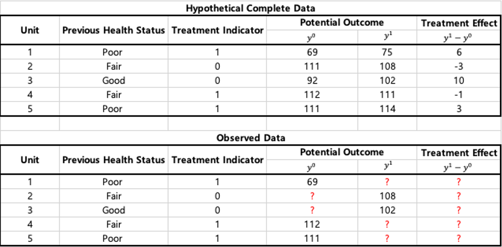
The ITE is identifiable under the hypothetical complete data.
In an observational setting, for someone assigned to the treatment condition, $y_i^1$ is observed and $y_i^0$ is the unobserved counterfactual outcome: it represents what would have happened to the individual if assigned to the control.
Thus, the fundamental problem of causal inference is that at most one of these two potential outcomes can be observed for each unit. We can never measure a causal effect directly, in the observational setting.

10.2.1 Ways of getting around

In the situation that outcomes at both conditions are not observed within each individual, we can never measure a causal effect directly.
Then we can think of causal inference as a prediction of what would happen to unit $i$ if $T_i=0$ or $T_i=1$ .
It is thus predictive inference in the potential-outcome framework.
Estimating causal effects requires one or some combination of the following:
- close substitutes for the potential outcomes
- randomization
- statistical adjustment

Close substitues

The objective of the causal inference can be the measurements of $y_i^0$ and $y_i^1$ on the same individual $i$ .
Example: suppose you want to measure the effect of a new diet by comparing your weight before the diet ( $y_i^0$ ) and your weight after the diet ( $\hat{y}_i^1$ ).
- Here, an assumption is that all other factors on weight are kept constant before and after.

Randomization

When we cannot compare treatment and control outcomes for the same units, we try to compare them on similar units.
Similarity can be attained by using randomization to decide the treatment assignment.

Statistical Adjustment

In many situations, it is not always possible to achieve close similarity between treatment groups in a causal study.
In observational studies, units often end up treated or not based on characteristics that are predictive of outcome of interest.
- Ex) men enter a job training program because they have low earnings and future earnings is the outcome of interest. Randomization in this case can be unethical or impractical.
When treatment and control groups are not similar, modeling or other forms of statistical adjustment can be used to fill in the gap.

10.3 Randomized experiments

We begin with the cleanest scenario, an experiment with units randomly assigned to receive treatment and control, and with the units as a random sample from a population of interest. The random sampling and random assignment assumption allow us to estimate the average causal effect of the treatment in the population based on regression modelling.

10.3.1 Average causal effects and randomized experiments

Although we cannot estimate individual-level causal effect, we can design studies to estimate the population average treatment effect: $ATE = \mathbb{E}(y_i^1 - y_i^0),$ for the units $i$ in a larger population.

This can be estimated under randomized experiment, where each unit has a positive chance of receiving each of the possible treatments.
Then the regression coefficient for $T$ corresponds to the causal effect of the treatment, among population represented by the $n$ units.
Thus, the control group mean can act as a counterfactual for the treatment group (and vice versa).

What if the $n_0+n_1$ units are selected nonrandomly from the population but the the treatment is assigned at random within this sample(e.g., clinical trials)?

In this case, causal inferences are still justified, but inferences no longer generalize to the entire population.
it is the inference to be appropriate to a hypothetical subpopulation from which the experimental subjects were drawn.
Further modeling is needed to generalize to any other population.
Causal inferences are merited for a specific sample or population is said to have internal validity.
When inferences are generalized to a broader population of interest the study is said to have external validity.

10.3.1.1 Example: showing children an education TV show

electric <- read.table("electric.dat", header=T)
attach(electric)

## plot the raw data
onlytext <- function(string){
  plot(0:1, 0:1, bty='n', type='n', xaxt='n', yaxt='n', xlab='', ylab='')
  text(0.5, 0.5, string, cex=1.2, font=2)
}
nf <- layout (matrix(c(0,1:14), 5, 3, byrow=TRUE), c(5, 10, 10),
             c(1, 5, 5, 5, 5), TRUE)
par (mar=c(.2,.2,.2,.2))
onlytext ('Test scores in control classes')
onlytext ('Test scores in treated classes')

par (mar=c(1,1,1,1), lwd=0.7)
for (j in 1:4){
  onlytext(paste ('Grade', j))
  hist (control.Posttest[Grade==j], breaks=seq(0,125,5), xaxt='n', yaxt='n',
    main=NULL, col="gray", ylim=c(0,10))
  axis(side=1, seq(0,125,50), line=-.25, cex.axis=1, mgp=c(1,.2,0), tck=0)
  text (2, 6.5, paste ("mean =", round (mean(control.Posttest[Grade==j]))), adj=0)
  text (2, 5, paste ("  sd =", round (sd(control.Posttest[Grade==j]))), adj=0)

  hist (treated.Posttest[Grade==j], breaks=seq(0,125,5), xaxt='n', yaxt='n',
    main=NULL, col="gray", ylim=c(0,10))
  axis(side=1, seq(0,125,50), line=-.25, cex.axis=1, mgp=c(1,.2,0), tck=0)
  text (2, 6.5, paste ("mean =", round (mean(treated.Posttest[Grade==j]))), adj=0)
  text (2, 5, paste ("  sd =", round (sd(treated.Posttest[Grade==j]))), adj=0)
}

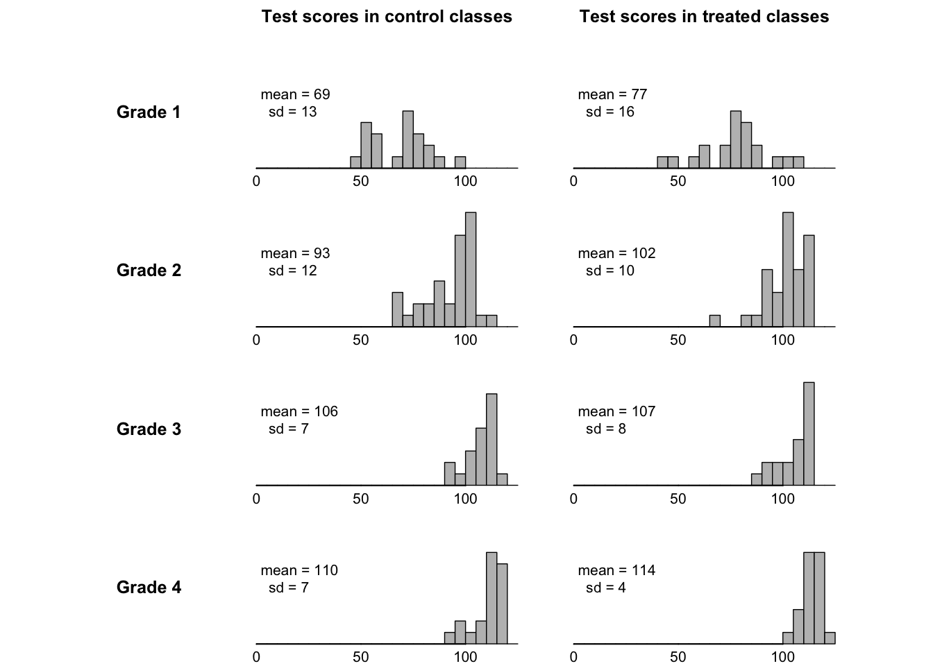
This figure summarizes data from an educational experiment performed around 1970 on a set of elementary school classes.

The treatment was exposure to a new education TV show called the Electric Company
In each of four grades, the classes were randomized into treated and control groups.
At the end of the school year, students were given a reading test and the average test score within each class was recorded (only class level data available)
Background:
- It is performed in two cities Fresno and Youngstown.
- For each city and grade, they selected a small number of schools (10-20), and within each school, they selected two poorest reading classes of that grade.
- For each pair, one of these classes was randomly assigned to continue with the control and treatment.
- This design is called paired comparisons design (the special case of randomized block design).

Analysis as a completely randomized experiment Here, we wll analyze the data as if the treatment assignment had been completely randomized within each grade (Ignore blocks).

When treatments are assigned completely at random, we can think of the different treatment groups as a set of random samples from a common population.
Then the the population average under each treatment, $\mathbb{y^0}$ and $\mathbb{y^1}$ can be estimated by the sample averages and the difference can estimate the population difference, that is the average causal effect.
Equivalently, we can estimate the sample averages via regression: $y_i = \beta_0 + \beta_0T_i + \epsilon_i.$

post.test <- c (treated.Posttest, control.Posttest)
pre.test <- c (treated.Pretest, control.Pretest)
grade <- rep (Grade, 2)
treatment <- rep (c(1,0), rep(length(treated.Posttest),2))
n <- length (post.test)

# output format to save
results <- data.frame(
  grade = integer(),
  estimate = numeric(),
  lower = numeric(),
  upper = numeric()
)

# For each grade save the ci
for (k in 1:4) {
  fit <- lm(post.test ~ treatment, subset = (grade == k))
  print(summary(fit))
  ci <- confint(fit)["treatment", ]
  coef <- coef(fit)["treatment"]
  
  results <- rbind(results, data.frame(
    grade = k,
    estimate = coef,
    lower = ci[1],
    upper = ci[2]
  ))
}

## 
## Call:
## lm(formula = post.test ~ treatment, subset = (grade == k))
## 
## Residuals:
##     Min      1Q  Median      3Q     Max 
## -32.890 -13.190   2.060   7.685  31.510 
## 
## Coefficients:
##             Estimate Std. Error t value Pr(>|t|)    
## (Intercept)   68.790      3.268  21.047   <2e-16 ***
## treatment      8.300      4.622   1.796   0.0801 .  
## ---
## Signif. codes:  0 '***' 0.001 '**' 0.01 '*' 0.05 '.' 0.1 ' ' 1
## 
## Residual standard error: 14.98 on 40 degrees of freedom
## Multiple R-squared:  0.0746, Adjusted R-squared:  0.05146 
## F-statistic: 3.224 on 1 and 40 DF,  p-value: 0.0801
## 
## 
## Call:
## lm(formula = post.test ~ treatment, subset = (grade == k))
## 
## Residuals:
##     Min      1Q  Median      3Q     Max 
## -35.171  -6.796   2.509   9.299  17.088 
## 
## Coefficients:
##             Estimate Std. Error t value Pr(>|t|)    
## (Intercept)   93.212      1.907   48.88  < 2e-16 ***
## treatment      8.359      2.697    3.10  0.00285 ** 
## ---
## Signif. codes:  0 '***' 0.001 '**' 0.01 '*' 0.05 '.' 0.1 ' ' 1
## 
## Residual standard error: 11.12 on 66 degrees of freedom
## Multiple R-squared:  0.1271, Adjusted R-squared:  0.1138 
## F-statistic: 9.607 on 1 and 66 DF,  p-value: 0.002848
## 
## 
## Call:
## lm(formula = post.test ~ treatment, subset = (grade == k))
## 
## Residuals:
##     Min      1Q  Median      3Q     Max 
## -17.610  -3.525   2.740   4.900   9.125 
## 
## Coefficients:
##             Estimate Std. Error t value Pr(>|t|)    
## (Intercept)  106.175      1.663  63.858   <2e-16 ***
## treatment      0.335      2.351   0.142    0.887    
## ---
## Signif. codes:  0 '***' 0.001 '**' 0.01 '*' 0.05 '.' 0.1 ' ' 1
## 
## Residual standard error: 7.436 on 38 degrees of freedom
## Multiple R-squared:  0.0005339,  Adjusted R-squared:  -0.02577 
## F-statistic: 0.0203 on 1 and 38 DF,  p-value: 0.8875
## 
## 
## Call:
## lm(formula = post.test ~ treatment, subset = (grade == k))
## 
## Residuals:
##     Min      1Q  Median      3Q     Max 
## -16.357  -1.489   1.093   3.918   7.933 
## 
## Coefficients:
##             Estimate Std. Error t value Pr(>|t|)    
## (Intercept)  110.357      1.299   84.98   <2e-16 ***
## treatment      3.710      1.837    2.02   0.0501 .  
## ---
## Signif. codes:  0 '***' 0.001 '**' 0.01 '*' 0.05 '.' 0.1 ' ' 1
## 
## Residual standard error: 5.951 on 40 degrees of freedom
## Multiple R-squared:  0.09255,    Adjusted R-squared:  0.06987 
## F-statistic:  4.08 on 1 and 40 DF,  p-value: 0.05014

# Visualization
ggplot(results, aes(x = factor(grade), y = estimate)) +
  geom_point(size = 3) +
  geom_errorbar(aes(ymin = lower, ymax = upper), width = 0.2) +
  labs(title = "Treatment Effect per Grade (95% CI)",
       x = "Grade",
       y = "Treatment Effect (Coefficient)") +
  theme_minimal()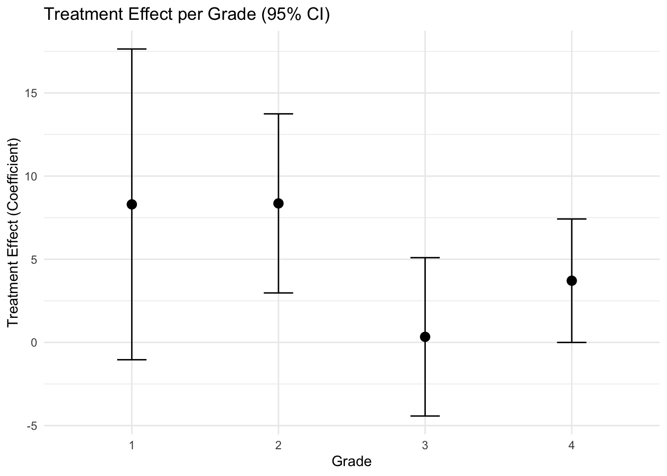

The treatemt appears to be effective, more in the second grade.

Controlling for pre-treatment predictors A pre-test was given in each class at the beginning(before treatment). We consider to include it in the model $y_i = \beta_0 + \beta_1T_i + \beta_2x_i+ \epsilon_i,$ where $x_i$ is the pre-treatment predictor.

Note. We avoid the term confouding covariates when describing adjustment in the context of randomized experiment. Predictors are included to increase precision since pre-test may affect the post-test, not the treatment assignment.

# output format to save
results <- data.frame(
  grade = integer(),
  estimate = numeric(),
  lower = numeric(),
  upper = numeric()
)

# For each grade save the ci
for (k in 1:4) {
  fit <- lm(post.test ~ treatment + pre.test, subset = (grade == k))
  print(summary(fit))
  ci <- confint(fit)["treatment", ]
  coef <- coef(fit)["treatment"]
  
  results <- rbind(results, data.frame(
    grade = k,
    estimate = coef,
    lower = ci[1],
    upper = ci[2]
  ))
}

## 
## Call:
## lm(formula = post.test ~ treatment + pre.test, subset = (grade == 
##     k))
## 
## Residuals:
##     Min      1Q  Median      3Q     Max 
## -19.360  -5.059   0.445   5.640  15.349 
## 
## Coefficients:
##             Estimate Std. Error t value Pr(>|t|)    
## (Intercept) -11.0229     8.7860  -1.255  0.21709    
## treatment     8.7865     2.6118   3.364  0.00173 ** 
## pre.test      5.1084     0.5498   9.292 1.96e-11 ***
## ---
## Signif. codes:  0 '***' 0.001 '**' 0.01 '*' 0.05 '.' 0.1 ' ' 1
## 
## Residual standard error: 8.461 on 39 degrees of freedom
## Multiple R-squared:  0.712,  Adjusted R-squared:  0.6973 
## F-statistic: 48.22 on 2 and 39 DF,  p-value: 2.863e-11
## 
## 
## Call:
## lm(formula = post.test ~ treatment + pre.test, subset = (grade == 
##     k))
## 
## Residuals:
##      Min       1Q   Median       3Q      Max 
## -15.8446  -3.4414   0.3449   3.8631  11.2716 
## 
## Coefficients:
##             Estimate Std. Error t value Pr(>|t|)    
## (Intercept) 37.42877    3.99098   9.378 1.07e-13 ***
## treatment    4.26577    1.35896   3.139  0.00255 ** 
## pre.test     0.78891    0.05486  14.382  < 2e-16 ***
## ---
## Signif. codes:  0 '***' 0.001 '**' 0.01 '*' 0.05 '.' 0.1 ' ' 1
## 
## Residual standard error: 5.479 on 65 degrees of freedom
## Multiple R-squared:  0.7913, Adjusted R-squared:  0.7848 
## F-statistic: 123.2 on 2 and 65 DF,  p-value: < 2.2e-16
## 
## 
## Call:
## lm(formula = post.test ~ treatment + pre.test, subset = (grade == 
##     k))
## 
## Residuals:
##     Min      1Q  Median      3Q     Max 
## -5.2063 -1.7614  0.3153  1.7005  6.9502 
## 
## Coefficients:
##             Estimate Std. Error t value Pr(>|t|)    
## (Intercept) 40.58424    3.72776   10.89  4.3e-13 ***
## treatment    1.90973    0.77616    2.46   0.0187 *  
## pre.test     0.68466    0.03849   17.79  < 2e-16 ***
## ---
## Signif. codes:  0 '***' 0.001 '**' 0.01 '*' 0.05 '.' 0.1 ' ' 1
## 
## Residual standard error: 2.438 on 37 degrees of freedom
## Multiple R-squared:  0.8953, Adjusted R-squared:  0.8897 
## F-statistic: 158.3 on 2 and 37 DF,  p-value: < 2.2e-16
## 
## 
## Call:
## lm(formula = post.test ~ treatment + pre.test, subset = (grade == 
##     k))
## 
## Residuals:
##     Min      1Q  Median      3Q     Max 
## -5.3504 -1.0094  0.0801  0.7166  7.0962 
## 
## Coefficients:
##             Estimate Std. Error t value Pr(>|t|)    
## (Intercept) 41.99473    4.28162   9.808 4.42e-12 ***
## treatment    1.70144    0.68535   2.483   0.0175 *  
## pre.test     0.65583    0.04082  16.066  < 2e-16 ***
## ---
## Signif. codes:  0 '***' 0.001 '**' 0.01 '*' 0.05 '.' 0.1 ' ' 1
## 
## Residual standard error: 2.184 on 39 degrees of freedom
## Multiple R-squared:  0.8809, Adjusted R-squared:  0.8748 
## F-statistic: 144.2 on 2 and 39 DF,  p-value: < 2.2e-16

# Visualization
ggplot(results, aes(x = factor(grade), y = estimate)) +
  geom_point(size = 3) +
  geom_errorbar(aes(ymin = lower, ymax = upper), width = 0.2) +
  labs(title = "Treatment Effect per Grade (95% CI)",
       x = "Grade",
       y = "Treatment Effect (Coefficient)") +
  theme_minimal()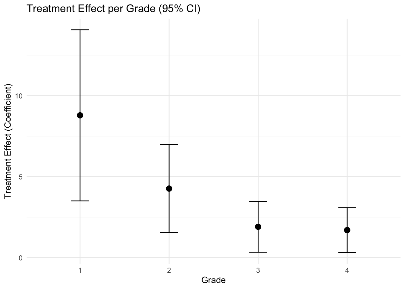

It is now clear that the treatment is effecitve, and it appears to be more efective in the lower grades.

Note It is only appropriate to control for pre-treatment predictors, or, more generally predictors that would not be affected by the treatment (such as age, gender..)

Transforming the outcome

We can transform the outcome variable to adjust for the pre-test scores: $g_i = postscore_i - prescore_i$ . And we can consider the model: $g_i = \beta_0 + \beta_1T_i+\epsilon_i$ to get the average difference of gain scores in treatment and control groups.

In some cases, this approach is more interpretable than the original variable.
However, it is valid when pre- score is comparable to post- score (e.g., the questions are different pre and post in the previous example).
Also, this approach is equivalent to setting the $\beta_2=1$ in the previous approach, which is an unnecessary assumption.
To resolve this, we can consider: $g_i = \beta_0 + \beta_1T_i + \beta_2x_i+ \epsilon_i$ . But this is equivalent to $y_i = \beta_0 + \beta_1T_i + \beta_2x_i+ \epsilon_i$ .

Modelling General treatment type

*When multiple treatments, the treatment effects can be defined relative to a baseline level. With random assignment, this simply follows general principles of regression modeling for causal infernece.

For numerical treatment levels, it can be considered as a continuous input.
To conceptualize, think of choosing a random number within predefined range.

SUTVA: Stable unit treatment value assumption

Consistency

There is a clearly defined, singular version of the treatment for each treatment condition
The treatment provided matches exactly the conceptual treatment intended in the study design

No interference

The treatment assignment for one unit does not affect the outcome of another – spillover or interference.
Otherwise, we would need to define a different potential outcome for the $i$ th unit not just for each treatment recieved by that unit but for each combination of treatment assignments received by every other unit in the experiment.
SUTVA is often violated in a spatial setting, region, family, social network.
Spatial interaction models explicitly model the dependency structure across space of units, allowing for controlled violations of the no-interferance assumption. For example: $y_i = \rho \sum_{j\neq i} \omega_{ij}y_j + \beta T_i + \epsilon_i$
- This includes splillover of treatments from neighbors, i.e., unit $i$ ’s outcome depends not only on its own treatment $T_i$ , but also on neighbor’s treatment $T_j$

10.3.2 Modelling with interaction

Let’s consider the three models for the previous example for grade 4:

fit1 = lm(post.test~treatment,subset=(grade==4))
fit2 = lm(post.test~treatment+pre.test,subset=(grade==4))
fit3 = lm(post.test~treatment+pre.test + treatment*pre.test,subset=(grade==4))

Consider first that with/without pretest models:

summary(fit1)

## 
## Call:
## lm(formula = post.test ~ treatment, subset = (grade == 4))
## 
## Residuals:
##     Min      1Q  Median      3Q     Max 
## -16.357  -1.489   1.093   3.918   7.933 
## 
## Coefficients:
##             Estimate Std. Error t value Pr(>|t|)    
## (Intercept)  110.357      1.299   84.98   <2e-16 ***
## treatment      3.710      1.837    2.02   0.0501 .  
## ---
## Signif. codes:  0 '***' 0.001 '**' 0.01 '*' 0.05 '.' 0.1 ' ' 1
## 
## Residual standard error: 5.951 on 40 degrees of freedom
## Multiple R-squared:  0.09255,    Adjusted R-squared:  0.06987 
## F-statistic:  4.08 on 1 and 40 DF,  p-value: 0.05014

summary(fit2)

## 
## Call:
## lm(formula = post.test ~ treatment + pre.test, subset = (grade == 
##     4))
## 
## Residuals:
##     Min      1Q  Median      3Q     Max 
## -5.3504 -1.0094  0.0801  0.7166  7.0962 
## 
## Coefficients:
##             Estimate Std. Error t value Pr(>|t|)    
## (Intercept) 41.99473    4.28162   9.808 4.42e-12 ***
## treatment    1.70144    0.68535   2.483   0.0175 *  
## pre.test     0.65583    0.04082  16.066  < 2e-16 ***
## ---
## Signif. codes:  0 '***' 0.001 '**' 0.01 '*' 0.05 '.' 0.1 ' ' 1
## 
## Residual standard error: 2.184 on 39 degrees of freedom
## Multiple R-squared:  0.8809, Adjusted R-squared:  0.8748 
## F-statistic: 144.2 on 2 and 39 DF,  p-value: < 2.2e-16

After ajusting for pretest, the treatment effect is 1.7.

Under a clean randomization, controlling for pre-treatment predictors should reduce the standard errors of the estimates.
If the randomization is less than clean, the addition of predictors may help us to control for unbalanced characteristics across groups.
Thus, this strategy has the potential to move us from estimating noncausal estimand due to lack of randomization to estimating a causal estimand by ‘cleaning’ the randomization.

Complicated arise when we include the interaction between treatment and pre-treatment predictors:

summary(fit3)

## 
## Call:
## lm(formula = post.test ~ treatment + pre.test + treatment * pre.test, 
##     subset = (grade == 4))
## 
## Residuals:
##     Min      1Q  Median      3Q     Max 
## -5.1894 -0.8621  0.2683  1.0329  6.3986 
## 
## Coefficients:
##                    Estimate Std. Error t value Pr(>|t|)    
## (Intercept)        37.84022    4.90126   7.721 2.66e-09 ***
## treatment          17.37223    9.60025   1.810   0.0783 .  
## pre.test            0.69569    0.04681  14.863  < 2e-16 ***
## treatment:pre.test -0.14718    0.08995  -1.636   0.1100    
## ---
## Signif. codes:  0 '***' 0.001 '**' 0.01 '*' 0.05 '.' 0.1 ' ' 1
## 
## Residual standard error: 2.138 on 38 degrees of freedom
## Multiple R-squared:  0.8887, Adjusted R-squared:  0.8799 
## F-statistic: 101.2 on 3 and 38 DF,  p-value: < 2.2e-16

The estimated treatment effect is $17.37-0.15x$ , which is hard to interpret without knowing the range of $x$ .

summary(pre.test[grade==4])

##    Min. 1st Qu.  Median    Mean 3rd Qu.    Max. 
##    78.4   104.2   107.3   105.8   110.8   119.8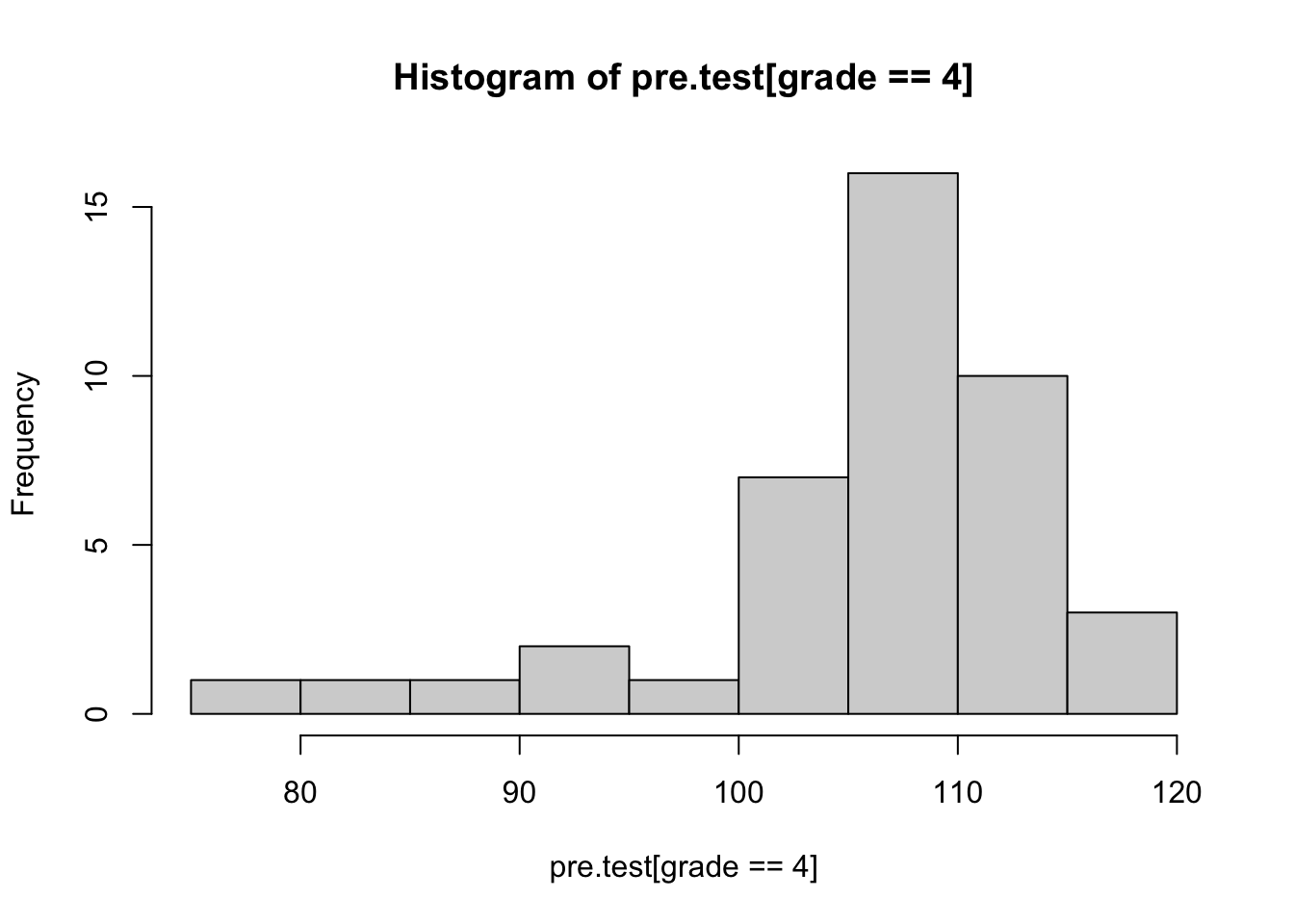

hist(pre.test[grade==4])

### The range of the causal effect
cc = coef(fit3)
cc[2] + cc[4] *  min(pre.test[grade==4]) # for mininum pretest

## treatment 
##  5.833014

cc[2] + cc[4] *  max(pre.test[grade==4]) # for maximum pretest

##  treatment 
## -0.2603968

## ploting
par (mfrow=c(1,1), mar=c(5,4,3,3))
lm.4.sim <- sim (fit3)
plot (0, 0, xlim=range (pre.test[grade==4]), ylim=c(-5,10),
       xlab="pre-test", ylab="treatment effect", main="treatment effect in grade 4")
abline (0, 0, lwd=.5, lty=2)
for (i in 1:20){
  curve (lm.4.sim@coef[i,2] + lm.4.sim@coef[i,4]*x, lwd=.5, col="gray", add=TRUE)}
curve (coef(fit3)[2] + coef(fit3)[4]*x, lwd=.5, add=TRUE)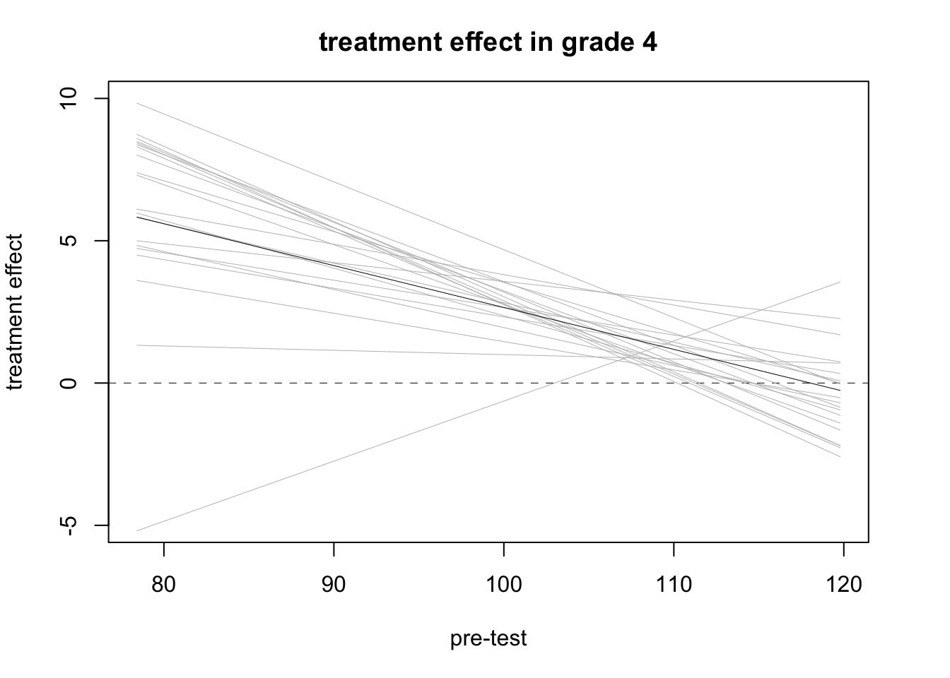

 # compute the average treatment effect & summarize

We can esimate a mean treatment effect by averaging over the values of $x$ in the data.

If we write the regression model: $y_i=\beta_0+\beta_1T_i + \beta_2 x_i +\epsilon_i$ , then the treatment effect becomes $\beta_1 +\beta_2 x$ . The summary treatment effect in the sample would be $\sum_{i=1}^n(\beta_1+\beta_2x_i)/n$ .

cc = coef(fit3)
mean(cc[2] + cc[4]*pre.test[grade==4])

## [1] 1.804733

n.sims <- nrow(lm.4.sim@coef)
effect <- array (NA, c(n.sims, sum(grade==4)))
for (i in 1:n.sims){
  effect[i,] <- lm.4.sim@coef[i,2] + lm.4.sim@coef[i,4]*pre.test[grade==4]
}
avg.effect <- rowMeans (effect)

print (c (mean(avg.effect), sd(avg.effect)))

## [1] 1.7689320 0.7331373

Or you can use the bootstrap approach for evaluating the standard error. The estimated causal effect of 1.8 is similar to the result without interaction term.

In general, for a linear regression model, the estimate obtained by including the interaction and then averaging over the data, reduces to the estimation without interaction.
Thus, modelling with interaction is to get a better idea of how the treatment effect varies with pre-treatment predictors, not simply to estimate an average effect.

10.3.3 Poststratification

In survey sampling, stratification refers to the procedure of dividing the population into disjoint subsets (strata), sampling separately within each stratum and then combining the stratum samples to get a population estimate.

Poststratification is the analysis of an unstratified sample, breaking the data into strata and reweighting as would have been done had the survey actually been stratified.
Stratification can adjust for potential differences between sample and population using the survey design; poststratification makes such adjustments in the data analysis step.

From the interaction model, we have discussed how treatment effects interact with pre-treatment predictors. To estimate an average treatment effect, we can post stratify- then average over the population.

For example, suppose we have treatment variable $T$ and pre-treatment variables $x_1$ and $x_2$ , the interaction model can be: $\hat{y} = \beta_0 + \beta_1 x_1 + \beta_2 x_2 + \beta_3 T + \beta_4 x_1T + \beta_5 x_2 T$
The estimated treatment effect is then $\beta_3 +\beta_4 x_1 + \beta_5 x_2$ .
Using population averages of $x_1$ and $x_2$ from available external source, we can compute the causal effect as $\beta_3 +\beta_4 \mu_1 + \beta_5 \mu_2$ . Or these can be replaced by sample averages of $x_1$ and $x_2$ . Simulation (Bootrap and Bayesian) can be used for estmating the standard error.

10.4 Observational studies

The simplest solution to the fundamental problem of causal inference is to randomly sample a different set of units for each treatment group from a common population. Equivalently, randomly assign the treatment among a selected set of units.

These approaches ensures that on average the different treatment groups are balanced
In other words, the $\bar{y}^0$ and $\bar{y}^1$ from the sample are estimating the average outcomes under control and treatment for the same population.

However, in observational studies, treatments are observed rather than assigned. It is not at all reasonable to consider the observed data under different treatments (e.g., smokers/nonsmokers) as random sample from a common population.

The example above had an embedded observational study.
Once the treatments had been assigned, the teacher for each class assigned to the treatment chose to either replace or supplement the regular reading program with the TV program.
Within the randomized treatment group, we focus on estimating the causal effect of replace/supplement on post-treatment test score.

supp <- c(ifelse(Supplement.=='S',1,0 ), rep(NA,nrow(electric)))

# output format to save
results <- data.frame(
  grade = integer(),
  estimate = numeric(),
  lower = numeric(),
  upper = numeric()
)

# For each grade save the ci
for (k in 1:4) {
  ok <- (grade==k) & (!is.na(supp))
  fit <- lm(post.test ~ supp + pre.test, subset = ok)
  print(summary(fit))
  ci <- confint(fit)["supp", ]
  coef <- coef(fit)["supp"]
  
  results <- rbind(results, data.frame(
    grade = k,
    estimate = coef,
    lower = ci[1],
    upper = ci[2]
  ))
}

## 
## Call:
## lm(formula = post.test ~ supp + pre.test, subset = ok)
## 
## Residuals:
##     Min      1Q  Median      3Q     Max 
## -21.999  -6.582  -0.485   6.908  14.055 
## 
## Coefficients:
##             Estimate Std. Error t value Pr(>|t|)    
## (Intercept)  -0.2160    12.1456  -0.018    0.986    
## supp          5.9230     4.4441   1.333    0.199    
## pre.test      4.7241     0.7846   6.021 1.08e-05 ***
## ---
## Signif. codes:  0 '***' 0.001 '**' 0.01 '*' 0.05 '.' 0.1 ' ' 1
## 
## Residual standard error: 9.42 on 18 degrees of freedom
## Multiple R-squared:  0.7035, Adjusted R-squared:  0.6706 
## F-statistic: 21.36 on 2 and 18 DF,  p-value: 1.769e-05
## 
## 
## Call:
## lm(formula = post.test ~ supp + pre.test, subset = ok)
## 
## Residuals:
##      Min       1Q   Median       3Q      Max 
## -13.2646  -2.8259  -0.8626   3.1002  12.7672 
## 
## Coefficients:
##             Estimate Std. Error t value Pr(>|t|)    
## (Intercept) 39.48608    6.52677   6.050 1.06e-06 ***
## supp         4.68689    1.83402   2.556   0.0157 *  
## pre.test     0.78168    0.08466   9.233 2.08e-10 ***
## ---
## Signif. codes:  0 '***' 0.001 '**' 0.01 '*' 0.05 '.' 0.1 ' ' 1
## 
## Residual standard error: 5.257 on 31 degrees of freedom
## Multiple R-squared:  0.7525, Adjusted R-squared:  0.7366 
## F-statistic: 47.13 on 2 and 31 DF,  p-value: 3.98e-10
## 
## 
## Call:
## lm(formula = post.test ~ supp + pre.test, subset = ok)
## 
## Residuals:
##    Min     1Q Median     3Q    Max 
## -6.180 -1.131  0.290  1.647  5.977 
## 
## Coefficients:
##             Estimate Std. Error t value Pr(>|t|)    
## (Intercept) 43.46910    6.23642   6.970 2.26e-06 ***
## supp        -1.29788    1.51307  -0.858    0.403    
## pre.test     0.68465    0.06245  10.963 3.96e-09 ***
## ---
## Signif. codes:  0 '***' 0.001 '**' 0.01 '*' 0.05 '.' 0.1 ' ' 1
## 
## Residual standard error: 2.848 on 17 degrees of freedom
## Multiple R-squared:  0.8864, Adjusted R-squared:  0.873 
## F-statistic: 66.32 on 2 and 17 DF,  p-value: 9.357e-09
## 
## 
## Call:
## lm(formula = post.test ~ supp + pre.test, subset = ok)
## 
## Residuals:
##     Min      1Q  Median      3Q     Max 
## -5.0600 -0.6256  0.3921  1.1380  6.2540 
## 
## Coefficients:
##             Estimate Std. Error t value Pr(>|t|)    
## (Intercept) 54.72928   10.11638   5.410 3.86e-05 ***
## supp        -0.32384    1.17112  -0.277    0.785    
## pre.test     0.55473    0.09541   5.814 1.65e-05 ***
## ---
## Signif. codes:  0 '***' 0.001 '**' 0.01 '*' 0.05 '.' 0.1 ' ' 1
## 
## Residual standard error: 2.581 on 18 degrees of freedom
## Multiple R-squared:  0.6609, Adjusted R-squared:  0.6232 
## F-statistic: 17.54 on 2 and 18 DF,  p-value: 5.936e-05

# Visualization
ggplot(results, aes(x = factor(grade), y = estimate)) +
  geom_point(size = 3) +
  geom_errorbar(aes(ymin = lower, ymax = upper), width = 0.2) +
  labs(title = "Supplement Effect per Grade (95% CI)",
       x = "Grade",
       y = "Supplement Effect (Coefficient)") +
  theme_minimal()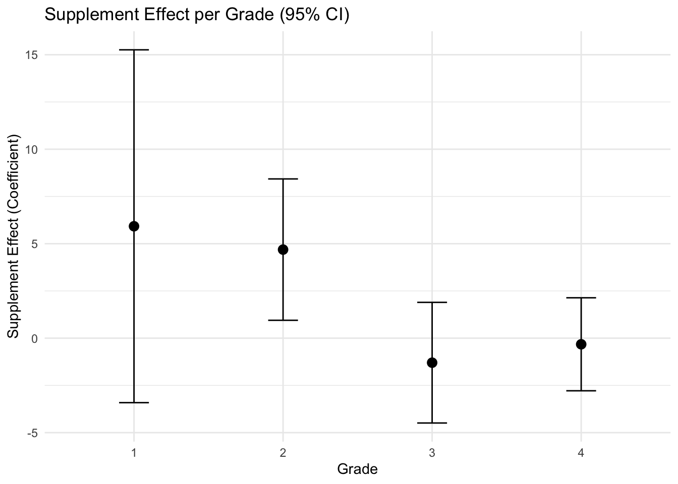

The uncertainties are high enough that the comparison is inconclusive except in grade 2, but the whole pattern is consistent with the reasonable hypothesis that supplementing is more effective than replacing in the lower grades.

Assumption of ignorable treatment assignment The key assumption for the causal effect under observational setting is that, conditional on the confounding covariates used in the analysis, the distribution units across treatment conditions is ‘random’ with respect to the potential outcomes. It can be expressed as: $y^0,y^1 \perp T | X$

The distribution of potential outcomes $(y^0,y^1)$ is the same across levels of the treatment variables, T, once we condition on confounding covariates $X$ .
In the example, we expect any two classes at the same levels of pre-treatment variables to have had the same probability of receiving supplemental version of the treatment.
It requires that we control for all confounding covariates, the pre-treatment variables that are associated with both the treatment and outcome.
If ignorability holds, then causal inference can be made without modeling the treatment assignment process.
non-ignorable assignment mechanism in the example:
1. if the teacher of each class chose the treatment that he/she believed would be more effective for that class based on unmeasured characteristics of the class that were related to their subsequent test scores.
2. if supplementing was more likely to be chosen by more motivated teachers, with teacher motivation also associated with the students’ future test score.
If teachers’ motivation might affect treatment assignment, it would be advisable to have a pre-treatment measure of teacher motivation and include as an input in the regression model. If not available, other proxies can be used (e.g.,years of experience)

10.5 Balance and Overlap

For causal inference, the units receiving the treatment should be comparable to those receiving the control.
For ignorable models, we consider two sorts of departures from comparability:
- Imbalance occurs if the distribution of relevant pre-treatment variables differ for the treatment and control groups
- lack of complete overlap occurs if there are regions in the space of pre-treatment variables where there are treated units but no controls, or controls but no treated units.
These should be checked with graphical display, calculating Standardized Difference in means and etc.

You will find techniques to solve these problems such as trimming, exact matching, propensity score matching, inverse probability of treatment weighting (IPTW) and etc, and causal inference in more complex (e.g., longitudinal) settings such as g-methods and marginal structural models(MSMs).

Also there are other general causal framework of mediation analysis and instrumental variable (IV) analysis.

Grolemund, Garrett. 2014. Hands-on Programming with r: Write Your Own Functions and Simulations. " O’Reilly Media, Inc.".

Matloff, Norman. 2011. The Art of r Programming: A Tour of Statistical Software Design. No Starch Press.

Wickham, Hadley, and Jennifer Bryan. 2023. R Packages. " O’Reilly Media, Inc.".

Wickham, Hadley, Mine Çetinkaya-Rundel, and Garrett Grolemund. 2023. R for Data Science. " O’Reilly Media, Inc.".