Chapter 6 Linear Regression: the advanced

It is not always appropriate to fit a classical linear regression model using data in their raw form. Let’s consider transformations and combinations, both in predictors and the outcome.

6.1 Linear transformation

Linear transformations do not affect the fit of a classical regression model, and they do not affect predictions: the changes in the inputs and the coefficients cancel informing the predicted value $X\beta$ .
However, well-chosen linear transformation can improve interpretability of coefficients.

6.1.1 Scaling of predictors and regression coefficients

The regression coefficient $\beta_j$ represents the average difference in $y$ comparing units that differ by 1 unit on the $j^{th}$ predictor. Sometimes a difference of 1 unit on the $x$ -scale is not the most relevant comparison.
Consider to predict earnings(in dollars) given their height (in inches) and sex (coded as 1 for men and 2 for women) from a survey of adult Americans in 1994.

library(foreign)
library ("arm")
library(tidyverse)
library(RColorBrewer)
heights <- read.dta ("files/GelmanData/heights.dta")
attach(heights)

df = data.frame(height=height,earn=earn,sex=factor(sex,labels=c('men','women')))
ggplot(df, aes(x = height, y = earn, color=sex)) +
  geom_point(alpha=0.5) +
  geom_smooth(method = "loess", se = F) +
  scale_color_manual(values = c("men" = "steelblue", "women" = "tomato")) +
  theme_minimal()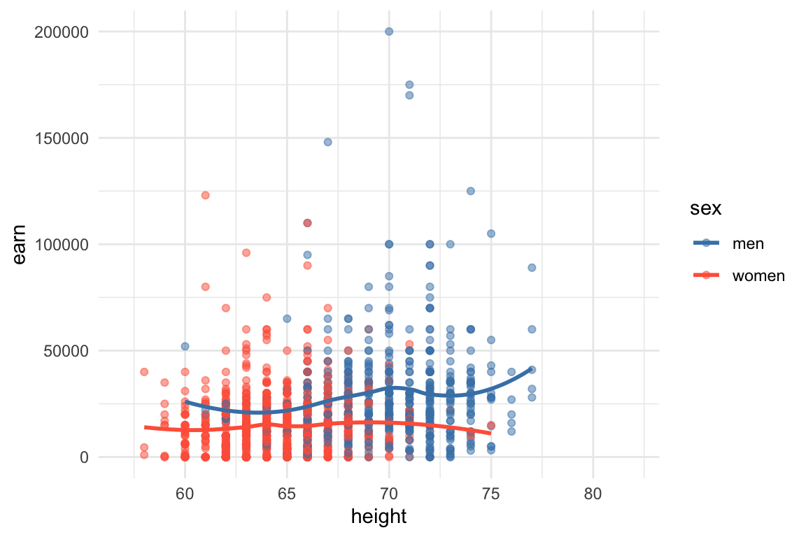

Let’s try linear model fit:

fit.full <- lm(earn~height*sex, data=df)
summary(fit.full)

## 
## Call:
## lm(formula = earn ~ height * sex, data = df)
## 
## Residuals:
##    Min     1Q Median     3Q    Max 
## -31209 -12591  -3172   7223 171109 
## 
## Coefficients:
##                 Estimate Std. Error t value Pr(>|t|)   
## (Intercept)     -25178.9    19281.3  -1.306  0.19181   
## height             772.4      275.0   2.809  0.00505 **
## sexwomen         16012.9    25099.3   0.638  0.52359   
## height:sexwomen   -403.7      371.0  -1.088  0.27670   
## ---
## Signif. codes:  0 '***' 0.001 '**' 0.01 '*' 0.05 '.' 0.1 ' ' 1
## 
## Residual standard error: 18460 on 1375 degrees of freedom
##   (650 observations deleted due to missingness)
## Multiple R-squared:  0.1296, Adjusted R-squared:  0.1277 
## F-statistic: 68.22 on 3 and 1375 DF,  p-value: < 2.2e-16

Write down the model fit?

fit1 <- update(fit.full,.~.-height:sex)
summary(fit1)

## 
## Call:
## lm(formula = earn ~ height + sex, data = df)
## 
## Residuals:
##    Min     1Q Median     3Q    Max 
## -30553 -12448  -3243   7451 171098 
## 
## Coefficients:
##             Estimate Std. Error t value Pr(>|t|)    
## (Intercept)  -9636.6    12953.7  -0.744  0.45705    
## height         550.5      184.6   2.983  0.00291 ** 
## sexwomen    -11254.6     1448.9  -7.768 1.55e-14 ***
## ---
## Signif. codes:  0 '***' 0.001 '**' 0.01 '*' 0.05 '.' 0.1 ' ' 1
## 
## Residual standard error: 18460 on 1376 degrees of freedom
##   (650 observations deleted due to missingness)
## Multiple R-squared:  0.1288, Adjusted R-squared:  0.1275 
## F-statistic: 101.7 on 2 and 1376 DF,  p-value: < 2.2e-16

anova(fit.full,fit1)

## Analysis of Variance Table
## 
## Model 1: earn ~ height * sex
## Model 2: earn ~ height + sex
##   Res.Df        RSS Df  Sum of Sq      F Pr(>F)
## 1   1375 4.6852e+11                            
## 2   1376 4.6892e+11 -1 -403495546 1.1842 0.2767

We stop here. The final model is: $earn = -9637 + 551\cdot height (inch) - 11255\cdot I(sex=Female) + error$

Change the interpretation to 1cm. It will be around 551/2.54?

# height transformed to cm
df_t <- df %>% mutate(height=height*2.54)
tfit <- lm(earn~height+sex,data=df_t) 
summary(tfit)

## 
## Call:
## lm(formula = earn ~ height + sex, data = df_t)
## 
## Residuals:
##    Min     1Q Median     3Q    Max 
## -30553 -12448  -3243   7451 171098 
## 
## Coefficients:
##              Estimate Std. Error t value Pr(>|t|)    
## (Intercept)  -9636.63   12953.75  -0.744  0.45705    
## height         216.75      72.67   2.983  0.00291 ** 
## sexwomen    -11254.57    1448.89  -7.768 1.55e-14 ***
## ---
## Signif. codes:  0 '***' 0.001 '**' 0.01 '*' 0.05 '.' 0.1 ' ' 1
## 
## Residual standard error: 18460 on 1376 degrees of freedom
##   (650 observations deleted due to missingness)
## Multiple R-squared:  0.1288, Adjusted R-squared:  0.1275 
## F-statistic: 101.7 on 2 and 1376 DF,  p-value: < 2.2e-16

The residual standard deviation and R-squared before and after transformation of the predictor do not change- linear transformation of the predictors does not affect the fit of a classical regression model.

6.1.2 Standardization using z-scores

Lets standardize the predictor:

df_s <- df %>% mutate(height=scale(height))
sfit <- lm(earn~height+sex,data=df_s) 
summary(sfit)

## 
## Call:
## lm(formula = earn ~ height + sex, data = df_s)
## 
## Residuals:
##    Min     1Q Median     3Q    Max 
## -30553 -12448  -3243   7451 171098 
## 
## Coefficients:
##             Estimate Std. Error t value Pr(>|t|)    
## (Intercept)    27008       1034  26.121  < 2e-16 ***
## height          2103        705   2.983  0.00291 ** 
## sexwomen      -11255       1449  -7.768 1.55e-14 ***
## ---
## Signif. codes:  0 '***' 0.001 '**' 0.01 '*' 0.05 '.' 0.1 ' ' 1
## 
## Residual standard error: 18460 on 1376 degrees of freedom
##   (650 observations deleted due to missingness)
## Multiple R-squared:  0.1288, Adjusted R-squared:  0.1275 
## F-statistic: 101.7 on 2 and 1376 DF,  p-value: < 2.2e-16

Then $\beta_1=2103$ will be interpreted in units of 1 sd of height. The intercept $\beta_0$ will be interpreted as the mean earning for male at the mean level of height.

6.2 Logarithmic transformations

When additivity and linearity are not reasonable assumptions, a nonlinear transformation can sometimes remedy the situation.

It commonly makes sense to take the logarithm of outcomes that are all positive.
This becomes clear when we make predictions on the original scale: the regression model imposes no constraints on predicted values
In that, we make prediction on log-scale and transform back by exponentiating ( $exp(a)>0$ for any real $a$ )
A linear model on the logarithmic scale corresponds to a multiplicative model on the original scale. $\log y_i = b_0 + b_1X_{i1} + b_2X_{i2} + \ldots +\epsilon_i$ This is equivalent to $y_i = e^{b_0 + b_1X_{i1} + b_2X_{i2} + \ldots +\epsilon_i}$ This can be expressed as $y_i = B_0\cdot B_1^{X_{i1}}\cdot B_2^{X_{i2}}\cdots E_i,$ with all positive $B_0,B_1,B_2,\ldots$ and $E_i$ .
Thus, on the scale of $y_i$ , the predictors come in multiplicatively.

6.2.1 Better models for earn~height

earn is positive outcome, it makes more sense in log-scale.

par(mfrow=c(1,2))
hist(earn);hist(log(earn))

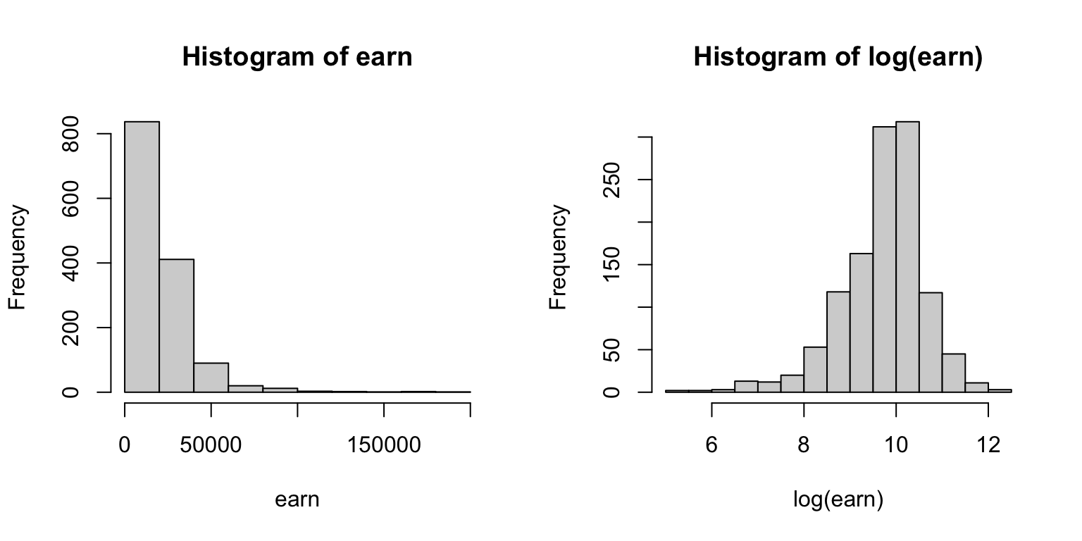
The previous inference was not correct anyways. Now consider the linear model in log scale.

df_log <- df %>% mutate(logearn=ifelse(earn==0,NA,log(earn)))
fit_log <- lm(logearn~height, data=df_log)
summary(fit_log)

## 
## Call:
## lm(formula = logearn ~ height, data = df_log)
## 
## Residuals:
##     Min      1Q  Median      3Q     Max 
## -4.4209 -0.3975  0.1394  0.5833  2.3536 
## 
## Coefficients:
##             Estimate Std. Error t value Pr(>|t|)    
## (Intercept) 5.778506   0.450927  12.815   <2e-16 ***
## height      0.058817   0.006728   8.743   <2e-16 ***
## ---
## Signif. codes:  0 '***' 0.001 '**' 0.01 '*' 0.05 '.' 0.1 ' ' 1
## 
## Residual standard error: 0.8931 on 1190 degrees of freedom
##   (837 observations deleted due to missingness)
## Multiple R-squared:  0.06035,    Adjusted R-squared:  0.05957 
## F-statistic: 76.44 on 1 and 1190 DF,  p-value: < 2.2e-16

Model:

The estimated slope was 0.06 which implies that a difference of 1 inch in height correspond to an expected 0.06 increase in log(earn).
So the original scale earn multiplied by $exp(0.06)\approx 1.06$ (Taylor expansion).
A difference of 1 inch in height corresponds to an expected positive difference of about 6% in the outcome variable.

6.2.2 Adding predictors

ggplot(df_log, aes(x = height, y = logearn, color=sex)) +
  geom_point(alpha=0.5) +
  geom_smooth(method = "loess", se = F) +
  scale_color_manual(values = c("men" = "steelblue", "women" = "tomato")) +
  theme_minimal()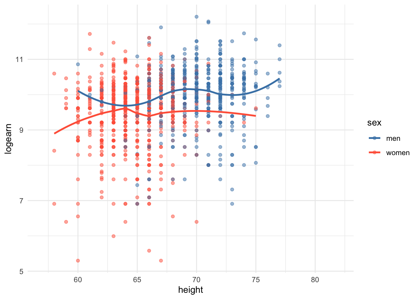

let’s include sex in the model.

lfit.ful <- lm(logearn ~ height*sex,data=df_log)
summary(lfit.ful)

## 
## Call:
## lm(formula = logearn ~ height * sex, data = df_log)
## 
## Residuals:
##     Min      1Q  Median      3Q     Max 
## -4.2297 -0.3720  0.1388  0.5646  2.2940 
## 
## Coefficients:
##                  Estimate Std. Error t value Pr(>|t|)    
## (Intercept)      8.309902   0.933098   8.906   <2e-16 ***
## height           0.024454   0.013306   1.838   0.0663 .  
## sexwomen         0.078586   1.257858   0.062   0.9502    
## height:sexwomen -0.007447   0.018635  -0.400   0.6895    
## ---
## Signif. codes:  0 '***' 0.001 '**' 0.01 '*' 0.05 '.' 0.1 ' ' 1
## 
## Residual standard error: 0.8812 on 1188 degrees of freedom
##   (837 observations deleted due to missingness)
## Multiple R-squared:  0.08668,    Adjusted R-squared:  0.08438 
## F-statistic: 37.58 on 3 and 1188 DF,  p-value: < 2.2e-16

lfit.r <- update(lfit.ful, .~.-height:sex)
summary(lfit.r)

## 
## Call:
## lm(formula = logearn ~ height + sex, data = df_log)
## 
## Residuals:
##     Min      1Q  Median      3Q     Max 
## -4.2384 -0.3718  0.1410  0.5649  2.3071 
## 
## Coefficients:
##              Estimate Std. Error t value Pr(>|t|)    
## (Intercept)  8.575907   0.653635  13.120  < 2e-16 ***
## height       0.020658   0.009312   2.218   0.0267 *  
## sexwomen    -0.423217   0.072462  -5.841 6.71e-09 ***
## ---
## Signif. codes:  0 '***' 0.001 '**' 0.01 '*' 0.05 '.' 0.1 ' ' 1
## 
## Residual standard error: 0.8809 on 1189 degrees of freedom
##   (837 observations deleted due to missingness)
## Multiple R-squared:  0.08656,    Adjusted R-squared:  0.08502 
## F-statistic: 56.34 on 2 and 1189 DF,  p-value: < 2.2e-16

anova(lfit.ful,lfit.r)

## Analysis of Variance Table
## 
## Model 1: logearn ~ height * sex
## Model 2: logearn ~ height + sex
##   Res.Df    RSS Df Sum of Sq      F Pr(>F)
## 1   1188 922.54                           
## 2   1189 922.67 -1    -0.124 0.1597 0.6895

Let’s set the main effects model as the final.

Interpretation:

Intercept= 8.576, This is the estimated log-earnings for a male (reference group for sex) with height = 0, which has no meaningful real-world interpretation since 0 height is not realistic. However, it serves as a baseline.
height: 0.02, After controlling for sex, a 1 unit increase in height is associated with about $100 \times (e^{0.02}-1)\approx 2%$ increase in earnings, on average.
women: -0.423, After controlling for height, women earn approximately $100\times (e^{-0.423}-1) \approx -34.5%$ less than men, on average.

However still I do not trust the model with only main effects with two reasons. (1) The scatterplot seperated by sex indicates stronger correlation between height and earn for men. (2) The models with and without interaction term, the slopes for sex and their significance (due to standard error) were drastically changed, which indicates that the procedure is unstable. So I am suspicious about strong multicollilinearity.

with(df_log,boxplot(height~sex))

with(df_log,wilcox.test(height~sex))

## 
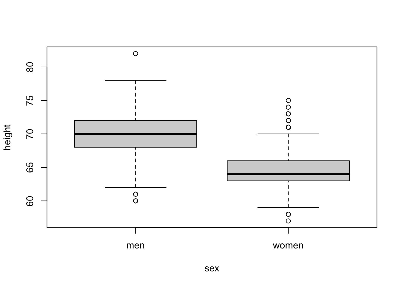
##  Wilcoxon rank sum test with continuity correction
## 
## data:  height by sex
## W = 875918, p-value < 2.2e-16
## alternative hypothesis: true location shift is not equal to 0

car::vif(lm(logearn~height+sex,data=df_log))

##   height      sex 
## 1.969404 1.969404

The vif was moderate but I still want to stabilize the procedure by centering height.

df_log_c <- df_log %>% mutate(cheight=scale(height,center=T,scale=F))
fit <- lm(logearn~cheight*sex,data=df_log_c)
summary(fit)

## 
## Call:
## lm(formula = logearn ~ cheight * sex, data = df_log_c)
## 
## Residuals:
##     Min      1Q  Median      3Q     Max 
## -4.2297 -0.3720  0.1388  0.5646  2.2940 
## 
## Coefficients:
##                   Estimate Std. Error t value Pr(>|t|)    
## (Intercept)       9.937620   0.060905 163.166  < 2e-16 ***
## cheight           0.024454   0.013306   1.838   0.0663 .  
## sexwomen         -0.417063   0.074106  -5.628 2.27e-08 ***
## cheight:sexwomen -0.007447   0.018635  -0.400   0.6895    
## ---
## Signif. codes:  0 '***' 0.001 '**' 0.01 '*' 0.05 '.' 0.1 ' ' 1
## 
## Residual standard error: 0.8812 on 1188 degrees of freedom
##   (837 observations deleted due to missingness)
## Multiple R-squared:  0.08668,    Adjusted R-squared:  0.08438 
## F-statistic: 37.58 on 3 and 1188 DF,  p-value: < 2.2e-16

Which model would you choose?

6.3 Adding polynomial terms

Or you can consider polynomial terms. It seems male and female have different nonlinear patterns between height and earn.

fit.poly <- lm(logearn ~ sex+ height + I(height^2) + sex:height + sex:I(height^2),data=df_log,x=TRUE,y=TRUE) # See x,y option for getting data matrix used
summary(fit.poly)

## 
## Call:
## lm(formula = logearn ~ sex + height + I(height^2) + sex:height + 
##     sex:I(height^2), data = df_log, x = TRUE, y = TRUE)
## 
## Residuals:
##     Min      1Q  Median      3Q     Max 
## -4.2445 -0.3639  0.1395  0.5566  2.3430 
## 
## Coefficients:
##                       Estimate Std. Error t value Pr(>|t|)
## (Intercept)          -8.057739  15.682270  -0.514    0.607
## sexwomen             -6.219562  21.240090  -0.293    0.770
## height                0.495802   0.451007   1.099    0.272
## I(height^2)          -0.003387   0.003240  -1.046    0.296
## sexwomen:height       0.219845   0.630768   0.349    0.727
## sexwomen:I(height^2) -0.001988   0.004690  -0.424    0.672
## 
## Residual standard error: 0.8806 on 1186 degrees of freedom
##   (837 observations deleted due to missingness)
## Multiple R-squared:  0.08945,    Adjusted R-squared:  0.08561 
## F-statistic:  23.3 on 5 and 1186 DF,  p-value: < 2.2e-16

df_log_fit <- data.frame(fit.poly$x,y=fit.poly$y,fitted=predict(fit.poly)) %>% 
              mutate(sex=factor(sexwomen,label=c('male','female'))) %>% 
              arrange(sex,height)

ggplot(df_log_fit, aes(x = height, y = y, color = sex)) +
  geom_point(alpha=0.5) +
  geom_line(aes(y = fitted), size = 1) +
  labs(title = "Fitted Lines by Sex",
       x = "Height", y = "Log(Earnings)") +
  theme_minimal()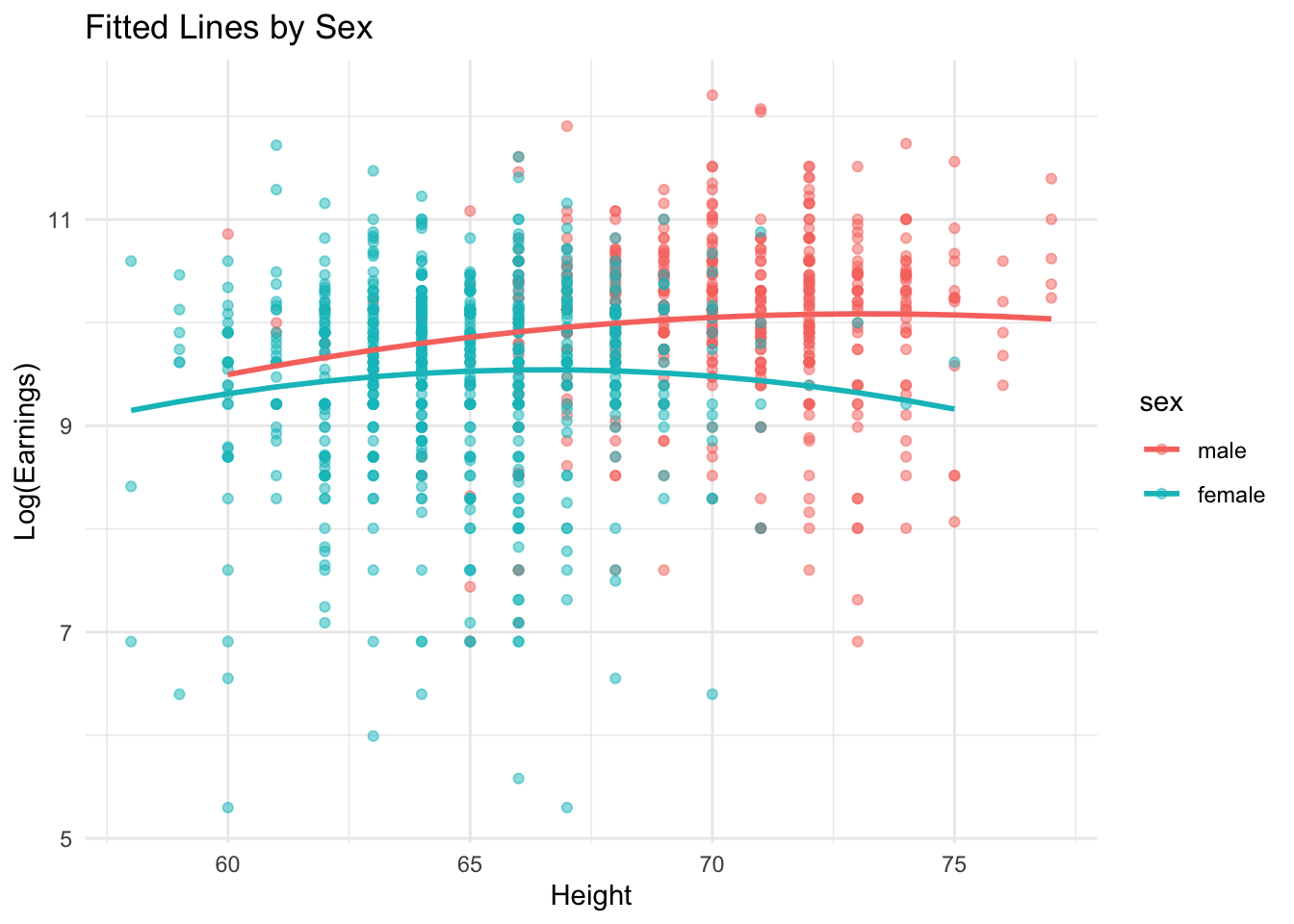

Consider higher order with the poly() function.

fit3 <- lm(logearn~poly(height,3,raw=T)*sex,data=df_log)
fit2 <- lm(logearn~poly(height,2,raw=T)*sex,data=df_log)
BIC(fit3,fit2)
anova(fit2,fit3)

Note We avoid discretizing continuous predictors (except as a way of simplifying a complicated transformation or to model nonlinearity). Transforming a continuous outcome to a binary outcome, for example, would discard much of the information in the data. However in some cases, it is appropriate to discretize a continuous variable if a simple monotonic or quadratic relation does not seem appropriate.

DIY Please select several of the model specifications we discussed (e.g., linear, polynomial, interaction models) and evaluate their predictive performance using the same dataset. I am particularly interested in whether modeling the outcome on the log scale results in improved prediction accuracy compared to using the original earnings scale. My initial hypothesis is that the log transformation will perform better.