Chapter 8 Generalized Linear Models

• Generalized linear modeling(GLM)* is a framework for statistical analysis that includes linear and logistic regression as special cases.

• A GLM involves a link function $g^{-1}$, yielding a vector of transformed data $\hat{y} = E(y) =g(X\beta)$.

• In linear regression, $g(u)=u$ (identity link).

• In logistic regression $g(u)=logit^{-1}(u)$, the logistic function.

8.1 Overview

1. The Poisson model is used for count data; that is, where each data point $y_i$ can equal $0,1,2,...$. The usual transformation of the linear combination of predictors is $g(u) = \exp(u)$. $y_i\sim Poisson$ is assumed. Poisson distribution has one parameter(same for mean and variance). Need an additional parameter to explain overdispersion.

2. The logistic-binomial model is used in settings where each data point $y_i$ represents the number of successes in some number $n_i$ trials. $n_i$ is not the same as $n$ the sample size. $y_i\sim Binomial(n_i,\pi_i)$ with $g(u)=logit^{-1}(u)$ and an overdispersion parameter.

3. The probit model is the same as logistic regression but with the logit function replaced by the normal cumulative distribution, or equivalently with the normal distribution instead of the logistic in the latent-data errors.

4. The Multinomial logit and probit models are extensions of logistic and probit regression for categorical data with more than two levels. These models use the logit or probit link function and the multinomial distribution is assumed with additional parameters to model the multi-categories. Multinomial models are further classified as $ordered$ or $unordered$.

5. Robust regression models replace the usual normal or logistic models by other distributions that allow occasional extreme values.

8.2 Poisson regression

• The Poisson distribution is used to model count data. In the model, each model $i$ corresponds to a setting (typically a spatial location or a time interval) in which $y_i$ events are observed. For example, $y_i$ could be the number of traffic accidents at intersection $i$ in a given year.

• In GLM framework, the variation in $y$ can be explained with linear combination of predictors $X$.

• For the traffic accident, the predictors could include a constant term, a measure of the average speed of traffic near the intersection, and an indicator for whether the intersection has a traffic signal.

• The basic Poisson model has the form: $$y_i\sim Poisson(\theta_i).$$

• The parameter $\theta_i$ must be positive. So it makes sense to fit a linear regression on the logarithmic scale: $$\theta_i = exp(X_i\beta),$$ which means we’re using a $log$ link.

• Example: $y_i\sim Poisson(e^{2.8+0.012X_{i1}-0.2X_{i2}})$, where $X_{i1}$ is average speed(mph), $X_{i2}=1$ if the intersection has a traffic signal.

  • The intercept is when both predictors are zero, which does not make sense. The slopes can be interpreted when other prdictors remains the same.

  • The coefficient of 0.012: $e^{0.12}=1.127$ tells that 12% increase in accident rate per ten mph.

  • The coefficient of -0.2: $e^{-0.2}=0.82$ tells that 18% reduction in accident rate when traffic signal.

8.2.1 Poisson regression with an exposure

• In most applications of Poissosn regression, the counts can be interpreted relative to ‘exposure’.

• For example, the number of vehicles that travel through the intersection.

• The poisson model with exposure $u_i$ for each sample $i$ is $$y_i = Poisson(u_i\theta_i).$$

• The poisson model is $\log(\theta_i) = X_i\beta +\log(u_i),$ where the logarithm of the exposure is called the offset in GLM terminology.

• So the poisson model with exposure is equivalent to including it as a regression predictor, but with its coefficient fixed to the value 1!

8.2.1.1 Differences between the binomial and Poisson models

Both are for count data but different application.

• If each data point $y_i$ can interpreted as the number of successes out of $n_i$ trials, then it is standard to use the binomial/logistic model (or its overdispersed generalization)

• If each data point $y_i$ does not have a natural limit- it is not based on a number of independent trials- then it is standard to use the Poisson/logarithmic regression model (or its overdispersed generalization).

8.2.1.2 Example: Poisson regression from simulated data using a table

data("VADeaths")
?VADeaths

You can see that there are three factors (Rural/Urban, Sex, age) on death rates measured per 1000 population per year. We’ll simulate counts and exposures using this rate table.

dat <- as.data.frame(as.table(VADeaths))

# the death table to data frame
region_sex <- matrix(unlist(strsplit(as.character(dat[,2]),' ')),byrow=T,ncol=2)
newdat = data.frame(dat[,1],region_sex,dat[,3])
colnames(newdat) <- c('Age','Region','Sex','Rate')

# Simulate population and death counts
set.seed(101)
n = nrow(newdat)
newdat$Population <- sample(800:1500,n,replace=TRUE)
newdat$Deaths <- round(newdat$Rate/1000 * newdat$Population)

head(newdat)

##     Age Region    Sex Rate Population Deaths
## 1 50-54  Rural   Male 11.7       1229     14
## 2 55-59  Rural   Male 18.1        894     16
## 3 60-64  Rural   Male 26.9       1008     27
## 4 65-69  Rural   Male 41.0       1241     51
## 5 70-74  Rural   Male 66.0       1150     76
## 6 50-54  Rural Female  8.7       1114     10

Let’s perform Poisson model with exposure.

fit <- glm(Deaths~Age + Region + Sex + offset(log(Population)), family=poisson, data=newdat)
summary(fit)

## 
## Call:
## glm(formula = Deaths ~ Age + Region + Sex + offset(log(Population)), 
##     family = poisson, data = newdat)
## 
## Coefficients:
##             Estimate Std. Error z value Pr(>|z|)    
## (Intercept) -4.76789    0.15180 -31.408  < 2e-16 ***
## Age55-59     0.42978    0.18526   2.320   0.0203 *  
## Age60-64     0.84703    0.16551   5.118 3.09e-07 ***
## Age65-69     1.30070    0.16016   8.121 4.62e-16 ***
## Age70-74     1.70452    0.15137  11.261  < 2e-16 ***
## RegionUrban  0.11803    0.07513   1.571   0.1162    
## SexMale      0.36400    0.07707   4.723 2.32e-06 ***
## ---
## Signif. codes:  0 '***' 0.001 '**' 0.01 '*' 0.05 '.' 0.1 ' ' 1
## 
## (Dispersion parameter for poisson family taken to be 1)
## 
##     Null deviance: 272.5166  on 19  degrees of freedom
## Residual deviance:   6.0615  on 13  degrees of freedom
## AIC: 123.73
## 
## Number of Fisher Scoring iterations: 4

The fitted model is: $$\log\theta_i = -4.8 + 0.4I(age_i \in 55-59) + 0.8I(age_i \in 60-64) + 1.3I(age_i \in 65-69)$$ $$+ 1.7I(age_i \in 70-74) + 0.1I(Region_i=Urban) + 0.4I(Sex_i=Male) +\log(Population_i)$$

• $\theta_i$ is the expected number of deaths in the cell $i$ in the death table

• offset(log(Population)) adjusts for the size of the population $\rightarrow$ modelling the motality rate per person

• Interpretation of the coefficients (IRR=incidence rate ratio):

exp(coef(fit))

## (Intercept)    Age55-59    Age60-64    Age65-69    Age70-74 RegionUrban     SexMale 
## 0.008498299 1.536912859 2.332707477 3.671853924 5.498745360 1.125281685 1.439075082

All slopes are interpreted after adjusting for all the other variables..

• Intercept: The death rate is 8 death per 1000 people for population aged 50-55, rural, Female

• Age 55-59: IRR= 1.53 $\rightarrow$ 53% higher death rate than 50-54

• Age 60-64: IRR= 2.33 $\rightarrow$ 133% higher death rate than 50-54

• Urban: IRR=1.13 $\rightarrow$ 13% higher death rate than rural

• Male: IRR=1.44 $\rightarrow$ 44% higher death rate than Female

8.2.2 Modeling Overdipersion

Under Poisson distribution the variance equals mean, which sometimes unintended restriction in the model. In the poisson model using exposure, $E(y_i)=Var(y_i)=u_i\theta_i$.

• We define the standardized residuals: $$z_i = \frac{y_i-\hat{y}_i}{sd(\hat{y}_i)}=\frac{y_i - u_i\hat{\theta}_i}{\sqrt{u_i\hat{\theta}_i}},$$ where $\hat{\theta}_i = e^{X_i\hat{\beta}}$.

  • If the Poisson model is true, then the $z_i$’s should be approximately independent (not exactly due to the modeling), each with mean 0 and standard deviation 1.

  • If there is overdispersion, we would expect the $z_i$’s to be larger, in absolute value, reflecting the extra variation beyond what is predicted under the Poisson model

• We can test for overdispersion by computing $\sum_{i=1}^n z_i^2 \sim \chi^2_{n-k}$ under the null, that account for $k$ regression coefficients.

• Since the chi-squared distribution has mean of $n-k$, the ratio $$\frac{\sum_{i=1}^n z_i^2}{n-k}$$ is a summary of the overdispersion in the data compared to the fitted model.

yhat = predict(fit,type='response')
z  = (newdat$Deaths - yhat)/sqrt(yhat)
dispersion = sum(z^2) / fit$df.residual

• If the dispersion is close to 1, no overdispersion (Poisson assumption OK)
• If the dispersion is >1.5 or 2, overdispersion
• If the dispersion <1, underdispersion (rare)

8.2.2.1 How to handle under- over-dispersion in Poisson?

We can fit an over-, under- dispersed model using the quasipoisson family: variance is allowed to scale with the mean, $Var(y_i)=\phi\cdot \theta_i$

fit.quasi <- glm(Deaths~Age + Region + Sex + offset(log(Population)), family=quasipoisson, data=newdat)
summary(fit.quasi)

## 
## Call:
## glm(formula = Deaths ~ Age + Region + Sex + offset(log(Population)), 
##     family = quasipoisson, data = newdat)
## 
## Coefficients:
##             Estimate Std. Error t value Pr(>|t|)    
## (Intercept) -4.76789    0.10437 -45.683 9.64e-16 ***
## Age55-59     0.42978    0.12737   3.374  0.00498 ** 
## Age60-64     0.84703    0.11379   7.444 4.88e-06 ***
## Age65-69     1.30070    0.11012  11.812 2.52e-08 ***
## Age70-74     1.70452    0.10407  16.379 4.64e-10 ***
## RegionUrban  0.11803    0.05165   2.285  0.03974 *  
## SexMale      0.36400    0.05298   6.870 1.14e-05 ***
## ---
## Signif. codes:  0 '***' 0.001 '**' 0.01 '*' 0.05 '.' 0.1 ' ' 1
## 
## (Dispersion parameter for quasipoisson family taken to be 0.4726886)
## 
##     Null deviance: 272.5166  on 19  degrees of freedom
## Residual deviance:   6.0615  on 13  degrees of freedom
## AIC: NA
## 
## Number of Fisher Scoring iterations: 4

Compare the regression coefficients and check the dispersion parameter.

When there is a sign of overdispersion, the negative-binaomial distribution that allows $Var(y_i)=\theta_i + \alpha\theta_i^2$ with the overdispersion parameter $\alpha>0$ can be used. The NB cannot model underdispersion case ($\alpha<0$).

library(MASS)
fit.nb <- glm.nb(Deaths~Age + Region + Sex + offset(log(Population)), data=newdat) 

## Warning in theta.ml(Y, mu, sum(w), w, limit = control$maxit, trace = control$trace > : iteration limit
## reached
## Warning in theta.ml(Y, mu, sum(w), w, limit = control$maxit, trace = control$trace > : iteration limit
## reached

See the warnings() due to the model misspecification.

DIY Implement fitting procedure for the Poisson and Quasipoisson. Check if your algorithm works well using simulation.

8.3 Logistic-binomial model

The logistic model can also be used for count data, using the binomial distribution to model the number of successes out of specified number of possibilities, with the probability of success being fit to a logistic regression.

Example: Using Contagious bovine pleuropneumonia (CBPP) data, we are modeling the proportion of cattle infected in different herds and time periods.

library(lme4)
data("cbpp")
head(cbpp)

##   herd incidence size period
## 1    1         2   14      1
## 2    1         3   12      2
## 3    1         4    9      3
## 4    1         0    5      4
## 5    2         3   22      1
## 6    2         1   18      2

For each of the combination, we know

• incidence: number infected
• size: total number of cattle

For each herd $h$ and period $t$, we label $n_{ht}$ as the total number of cattle and $y_{ht}$ as the number of infected. Our model has the form: $$y_{ht} \sim Binomial(n_{ht},\pi_{ht})$$ $$\pi_{ht}=logit^{-1}(X_{ht}\beta).$$ where subscripts $h$ for herd and $t$ for time period.

Or, we can consider to include the time period as a categorical variable:

\[p_{st} = logit^{-1}(\mu +\alpha_h +\beta_1 I(t=2) + \beta_2 I(t=3) + \beta_3 I(t=4)).\]

Fit a logistic-binomial model for the incidence(count) data.

# The
dat <- cbpp %>% mutate(fail = size-incidence)

# handle time as a continuous
fit_glm1 <- glm(cbind(incidence,fail)~as.numeric(period) + herd, family=binomial(link='logit'),data=dat)
summary(fit_glm1)

## 
## Call:
## glm(formula = cbind(incidence, fail) ~ as.numeric(period) + herd, 
##     family = binomial(link = "logit"), data = dat)
## 
## Coefficients:
##                    Estimate Std. Error z value Pr(>|z|)    
## (Intercept)         -0.2258     0.4492  -0.503  0.61523    
## as.numeric(period)  -0.5110     0.1246  -4.100 4.12e-05 ***
## herd2               -1.2520     0.6085  -2.057  0.03964 *  
## herd3               -0.2789     0.5037  -0.554  0.57973    
## herd4               -0.7486     0.6626  -1.130  0.25860    
## herd5               -1.1164     0.5780  -1.931  0.05342 .  
## herd6               -1.4396     0.6473  -2.224  0.02615 *  
## herd7                0.3784     0.5242   0.722  0.47034    
## herd8                0.1306     0.5376   0.243  0.80803    
## herd9               -1.2984     0.8346  -1.556  0.11975    
## herd10              -1.6517     0.6446  -2.562  0.01039 *  
## herd11              -0.9276     0.5245  -1.769  0.07696 .  
## herd12              -0.9225     0.7279  -1.267  0.20503    
## herd13              -1.9737     0.7058  -2.796  0.00517 ** 
## herd14               0.6711     0.5635   1.191  0.23370    
## herd15              -1.7039     0.7097  -2.401  0.01635 *  
## ---
## Signif. codes:  0 '***' 0.001 '**' 0.01 '*' 0.05 '.' 0.1 ' ' 1
## 
## (Dispersion parameter for binomial family taken to be 1)
## 
##     Null deviance: 154.817  on 55  degrees of freedom
## Residual deviance:  70.684  on 40  degrees of freedom
## AIC: 186.64
## 
## Number of Fisher Scoring iterations: 5

# handle time as a categorical
fit_glm2 <- glm(cbind(incidence,fail)~period + herd, family=binomial(link='logit'),data=dat)
summary(fit_glm2)

## 
## Call:
## glm(formula = cbind(incidence, fail) ~ period + herd, family = binomial(link = "logit"), 
##     data = dat)
## 
## Coefficients:
##             Estimate Std. Error z value Pr(>|z|)    
## (Intercept) -0.62948    0.40901  -1.539 0.123796    
## period2     -0.89358    0.31311  -2.854 0.004319 ** 
## period3     -1.03164    0.33247  -3.103 0.001916 ** 
## period4     -1.46420    0.43320  -3.380 0.000725 ***
## herd2       -1.26236    0.61152  -2.064 0.038991 *  
## herd3       -0.31023    0.50650  -0.613 0.540203    
## herd4       -0.75457    0.66488  -1.135 0.256420    
## herd5       -1.09781    0.58079  -1.890 0.058731 .  
## herd6       -1.46224    0.64923  -2.252 0.024305 *  
## herd7        0.36177    0.52673   0.687 0.492201    
## herd8        0.02335    0.54413   0.043 0.965778    
## herd9       -1.33594    0.83684  -1.596 0.110396    
## herd10      -1.66818    0.64662  -2.580 0.009885 ** 
## herd11      -0.93448    0.52655  -1.775 0.075943 .  
## herd12      -0.93803    0.73059  -1.284 0.199165    
## herd13      -1.98378    0.70756  -2.804 0.005052 ** 
## herd14       0.58893    0.56845   1.036 0.300187    
## herd15      -1.73268    0.71175  -2.434 0.014916 *  
## ---
## Signif. codes:  0 '***' 0.001 '**' 0.01 '*' 0.05 '.' 0.1 ' ' 1
## 
## (Dispersion parameter for binomial family taken to be 1)
## 
##     Null deviance: 154.817  on 55  degrees of freedom
## Residual deviance:  68.826  on 38  degrees of freedom
## AIC: 188.78
## 
## Number of Fisher Scoring iterations: 5

BIC(fit_glm1,fit_glm2)

##          df      BIC
## fit_glm1 16 219.0461
## fit_glm2 18 225.2390

Handling the period as a continuos gives lower BIC value.

Additionally, it looks like herd10 has different probability of infection. However. overall, there is not much herd effect. So you can consider to remove the herd predictor. ### Modeling Overdispersion * When logistic regression is applied to count data, it is usual for the data to have more variation than is explained by the model due to the lack of the variance parameter.

• The mean of $y$ is $n\pi$ and variance is $n\pi(1-\pi)$.

• Similar to the Poisson model, we define the standardized residual for each data point $i$ as $$z_i = \frac{y_i-\hat{y}_i}{sd(\hat{y}_i)},$$ $$=\frac{y_i - n_i\hat{\pi}_i}{\sqrt{n_i\hat{\pi}_i(1-\hat{\pi}_i)}}.$$

• Then we compute the estimate overdispersion under assumption of the model fit: $$\sum_{i=1}^n z_i^2 / (n-k)$$

Or formally testing for the overdispersion using $\sum_{i=1}^n z_i^2 \sim \chi^2_{n-k}$, where $n$ here is the number of data points (differen from $n_i$).

pihat = predict(fit_glm1, type="response")
nn = (dat$incidence+dat$fail)
z  = (dat$incidence - nn*pihat)/sqrt(nn*pihat*(1-pihat))

sum(z^2) / fit_glm1$df.residual # dispersion

## [1] 1.570664

pchisq(sum(z^2),fit_glm1$df.residual,lower.tail=F) # pvalue

## [1] 0.01207116

Overdispersion happens. Let’s consider overdispersed models. The quasibinomical model assumes extra parameter $\omega$ for overdispersion: $Var(y_i) = \omega n_i\pi_i(1-\pi_i)$.

qfit_glm1 <- glm(cbind(incidence,fail)~as.numeric(period) + herd, family=quasibinomial(link='logit'),data=dat)
summary(qfit_glm1)

## 
## Call:
## glm(formula = cbind(incidence, fail) ~ as.numeric(period) + herd, 
##     family = quasibinomial(link = "logit"), data = dat)
## 
## Coefficients:
##                    Estimate Std. Error t value Pr(>|t|)   
## (Intercept)         -0.2258     0.5629  -0.401  0.69051   
## as.numeric(period)  -0.5110     0.1562  -3.272  0.00221 **
## herd2               -1.2520     0.7627  -1.642  0.10850   
## herd3               -0.2789     0.6313  -0.442  0.66096   
## herd4               -0.7486     0.8304  -0.901  0.37277   
## herd5               -1.1164     0.7244  -1.541  0.13115   
## herd6               -1.4396     0.8112  -1.775  0.08357 . 
## herd7                0.3784     0.6569   0.576  0.56781   
## herd8                0.1306     0.6737   0.194  0.84726   
## herd9               -1.2984     1.0459  -1.241  0.22169   
## herd10              -1.6517     0.8079  -2.045  0.04752 * 
## herd11              -0.9276     0.6573  -1.411  0.16592   
## herd12              -0.9225     0.9123  -1.011  0.31798   
## herd13              -1.9737     0.8846  -2.231  0.03133 * 
## herd14               0.6711     0.7062   0.950  0.34770   
## herd15              -1.7039     0.8894  -1.916  0.06257 . 
## ---
## Signif. codes:  0 '***' 0.001 '**' 0.01 '*' 0.05 '.' 0.1 ' ' 1
## 
## (Dispersion parameter for quasibinomial family taken to be 1.570667)
## 
##     Null deviance: 154.817  on 55  degrees of freedom
## Residual deviance:  70.684  on 40  degrees of freedom
## AIC: NA
## 
## Number of Fisher Scoring iterations: 5

# Consider to remove the herd factor
qfit_glm1_r <- glm(cbind(incidence,fail)~as.numeric(period), family=quasibinomial(link='logit'),data=dat)
anova(qfit_glm1,qfit_glm1_r)

## Analysis of Deviance Table
## 
## Model 1: cbind(incidence, fail) ~ as.numeric(period) + herd
## Model 2: cbind(incidence, fail) ~ as.numeric(period)
##   Resid. Df Resid. Dev  Df Deviance      F  Pr(>F)  
## 1        40     70.684                              
## 2        54    118.248 -14  -47.564 2.1631 0.02849 *
## ---
## Signif. codes:  0 '***' 0.001 '**' 0.01 '*' 0.05 '.' 0.1 ' ' 1

Note

• Logistic regression for binary data is a special case of this model with $n_i=1$ for all $i$. Overdispersion at the level of the individual data points cannot occur in the binary model.

• The binomial logistic model can be modeld in the binary data by considering each of the $n_i$ cases as a separate data point. The sample size in this case is $\sum_i n_i$. In this parameterization, overdispersion could be included in a multilevel model by considering herd as clusters.

8.4 Probit regression

The probit model is used for modeling binary data like logistic regression. We can write the model as $$P(y_i=1) = \Phi(X_i\beta),$$ where $\Phi$ is the normal cumulative distribution function. In the latent-data formulation, $$y_i = I(z_i>0),$$ $$z_i = X_i\beta +\epsilon_i,$$ $$\epsilon_i \sim N(0,1).$$

More generally, the model can have an error variance $\epsilon_i\sim N(0,\sigma^2)$. However $\sigma$ is not identifiable so we fix it to 1.

8.4.1 Probit vs. Logit?

# Define input range
x <- seq(-6, 6, length.out = 500)

# Compute logistic and probit (normal CDF) values
logistic <- 1 / (1 + exp(-x))
probit <- pnorm(x)

# Combine into data frame
df <- data.frame(x = x, Logistic = logistic, Probit = probit)

# Plot using ggplot2
library(ggplot2)
library(tidyr)

df_long <- pivot_longer(df, cols = c("Logistic", "Probit"), names_to = "Model", values_to = "Probability")

ggplot(df_long, aes(x = x, y = Probability, color = Model)) +
  geom_line(size = 1) +
  theme_minimal(base_size = 14) +
  labs(
    title = "Logistic vs Probit Link Functions",
    x = "Linear Predictor (x)",
    y = "Cumulative Probability"
  )

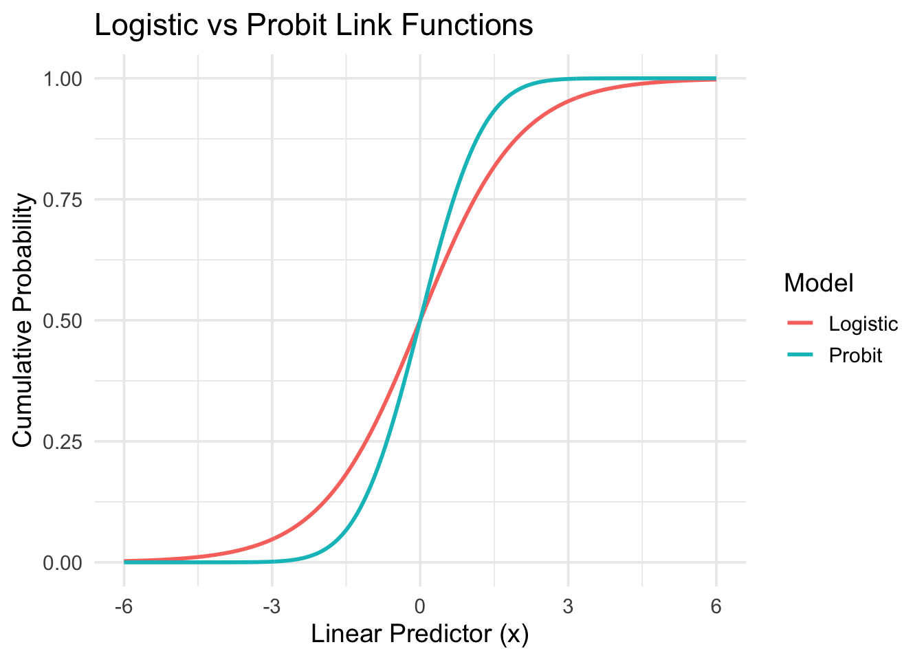
The shapes look pretty similar. However, the probit model is less interpretable in terms of odds and interpreted as linear effect on the latent factor $z$.

wells <- read.table ("files/GelmanData/wells.dat")
attach(wells)

## The following objects are masked from wells (pos = 3):
## 
##     arsenic, assoc, dist, educ, switch

dat <- wells %>% mutate(dist100 = dist/100)

fit_logistic <- glm (switch ~ dist100, family=binomial(link='logit'),data=dat)
summary(fit_logistic)

## 
## Call:
## glm(formula = switch ~ dist100, family = binomial(link = "logit"), 
##     data = dat)
## 
## Coefficients:
##             Estimate Std. Error z value Pr(>|z|)    
## (Intercept)  0.60596    0.06031  10.047  < 2e-16 ***
## dist100     -0.62188    0.09743  -6.383 1.74e-10 ***
## ---
## Signif. codes:  0 '***' 0.001 '**' 0.01 '*' 0.05 '.' 0.1 ' ' 1
## 
## (Dispersion parameter for binomial family taken to be 1)
## 
##     Null deviance: 4118.1  on 3019  degrees of freedom
## Residual deviance: 4076.2  on 3018  degrees of freedom
## AIC: 4080.2
## 
## Number of Fisher Scoring iterations: 4

fit_probit <- glm (switch ~ dist100, family=binomial(link='probit'),data=dat)
summary(fit_probit)

## 
## Call:
## glm(formula = switch ~ dist100, family = binomial(link = "probit"), 
##     data = dat)
## 
## Coefficients:
##             Estimate Std. Error z value Pr(>|z|)    
## (Intercept)  0.37781    0.03730   10.13  < 2e-16 ***
## dist100     -0.38741    0.06034   -6.42 1.36e-10 ***
## ---
## Signif. codes:  0 '***' 0.001 '**' 0.01 '*' 0.05 '.' 0.1 ' ' 1
## 
## (Dispersion parameter for binomial family taken to be 1)
## 
##     Null deviance: 4118.1  on 3019  degrees of freedom
## Residual deviance: 4076.3  on 3018  degrees of freedom
## AIC: 4080.3
## 
## Number of Fisher Scoring iterations: 4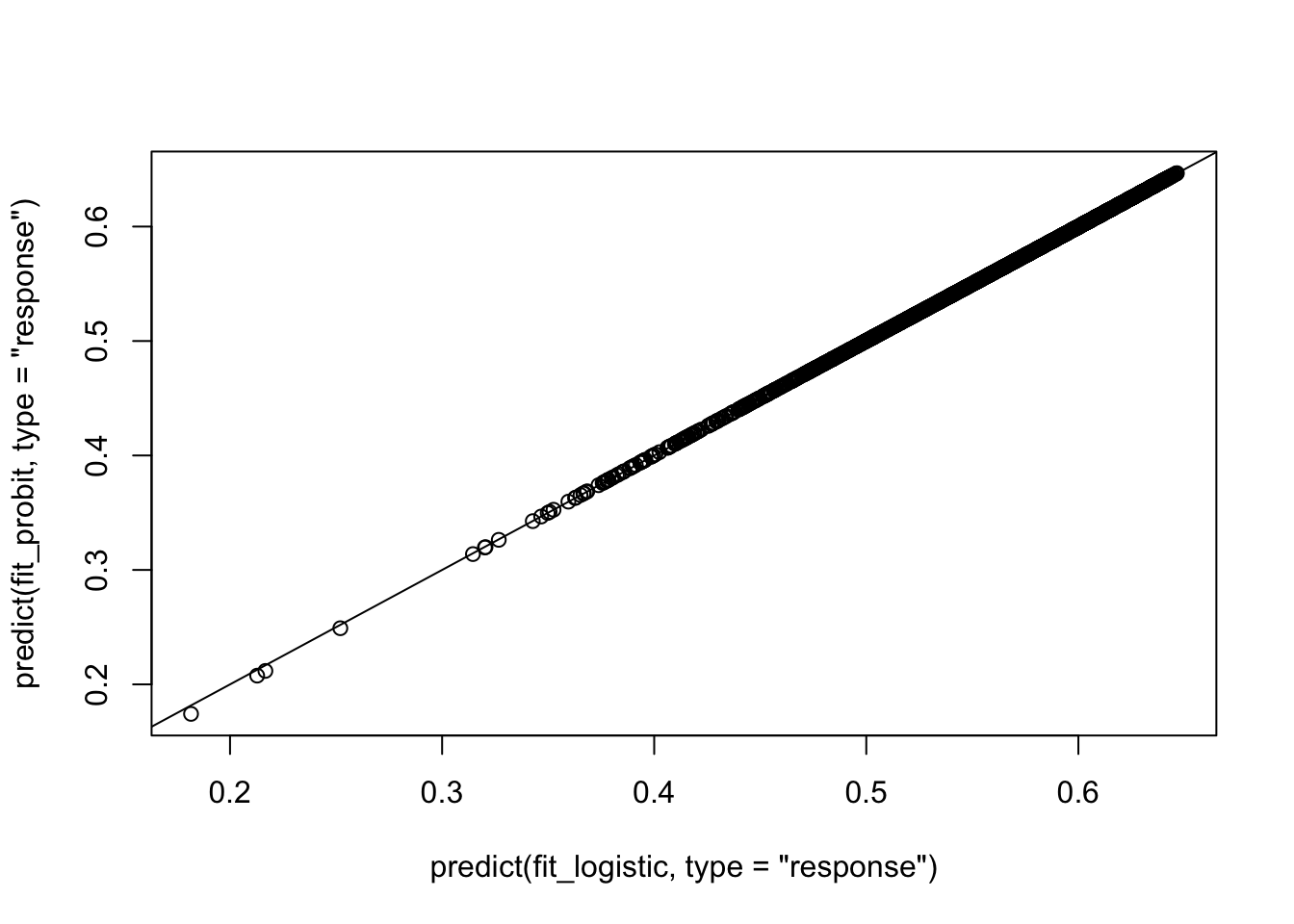

plot(predict(fit_logistic,type='response'),predict(fit_probit,type='response'))
abline(0,1)

As you see here, in terms of predicting $P(y=1)$, they are equiavalent. In that $$P(y_i=1) = \Phi(X_i\beta) \approx logit^{-1}(1.6(X_i\beta)).$$

DIY: Derive the equivalence.

8.5 Categorical regression

Logistic and probit regression can be extended to multiple categories, which can be ordered or unordered.

8.5.1 The ordered multinomial logit model

Consider a categorical outcome $y$ that cann take on the values $1,2,\ldots, K$. We can express it as a series of logistic regressions:

$$P(y>1) = logit^{-1}(X\beta-c_1)$$ $$P(y>2) = logit^{-1}(X\beta-c_2)$$ $$P(y>3) = logit^{-1}(X\beta-c_3)$$ $$\vdots$$ $$P(y>K-1) = logit^{-1}(X\beta-c_{K-1}).$$

• The parameters $c_k$ (called thresholds or cutpoints) are constrained to increase: $c_1<c_2<\cdots<c_{K-1},$ because the probabilities are stricktly decreasing.
• The model with $K$ categories has $K-2$ parameters for $c_k$ in addition to $\beta$.
• The cutpoints $c_2,\ldots,c_{K-1}$ can be estimated using the maximum likelihood, simultaneously with the coefficients $\beta$.
• From the model, we can compute the probabilities of individual outcomes: $$P(y=k) = Pr(y>k-1) - P(y>k)$$ $$= logit^{-1}(X\beta - c_{k-1}) - logit^{-1}(X\beta-c_k)$$
• To interpret the regression coefficients, the model can be expressed as odds: $$\log\frac{P(y\leq k)}{P(y>k)}=logit(P(y\leq k))=c_k-X\beta.$$

8.5.1.1 Example

A study looks at factors that influence the decision of whether to apply to graduate school. College juniors are asked if they are unlikely, somewhat likely, or very likely to apply to graduate school. Hence, our outcome variable has three categories. Data on parental educational status, whether the undergraduate institution is public or private, and current GPA is also collected. The researchers have reason to believe that the “distances” between these three points are not equal. For example, the “distance” between “unlikely” and “somewhat likely” may be shorter than the distance between “somewhat likely” and “very likely”.

require(foreign)
dat <- read.dta("https://stats.idre.ucla.edu/stat/data/ologit.dta")
head(dat)

##             apply pared public  gpa
## 1     very likely     0      0 3.26
## 2 somewhat likely     1      0 3.21
## 3        unlikely     1      1 3.94
## 4 somewhat likely     0      0 2.81
## 5 somewhat likely     0      0 2.53
## 6        unlikely     0      1 2.59

This hypothetical data set has a three level variable called apply, with levels “unlikely”, “somewhat likely”, and “very likely”, coded 1, 2, and 3, respectively, that we will use as our outcome variable. We also have three variables that we will use as predictors: pared, which is a 0/1 variable indicating whether at least one parent has a graduate degree; public, which is a 0/1 variable where 1 indicates that the undergraduate institution is public and 0 private, and gpa, which is the student’s grade point average. Let’s start with the descriptive statistics of these variables.

lapply(dat[, c("apply", "pared", "public")], table)

## $apply
## 
##        unlikely somewhat likely     very likely 
##             220             140              40 
## 
## $pared
## 
##   0   1 
## 337  63 
## 
## $public
## 
##   0   1 
## 343  57

ftable(xtabs(~ public + apply + pared, data = dat))

##                        pared   0   1
## public apply                        
## 0      unlikely              175  14
##        somewhat likely        98  26
##        very likely            20  10
## 1      unlikely               25   6
##        somewhat likely        12   4
##        very likely             7   3

summary(dat$gpa)

##    Min. 1st Qu.  Median    Mean 3rd Qu.    Max. 
##   1.900   2.720   2.990   2.999   3.270   4.000

ggplot(dat, aes(x = apply, y = gpa)) +
  geom_boxplot(size = .75) +
  geom_jitter(alpha = .5) +
  facet_grid(pared ~ public, margins = TRUE) +
  theme(axis.text.x = element_text(angle = 45, hjust = 1, vjust = 1))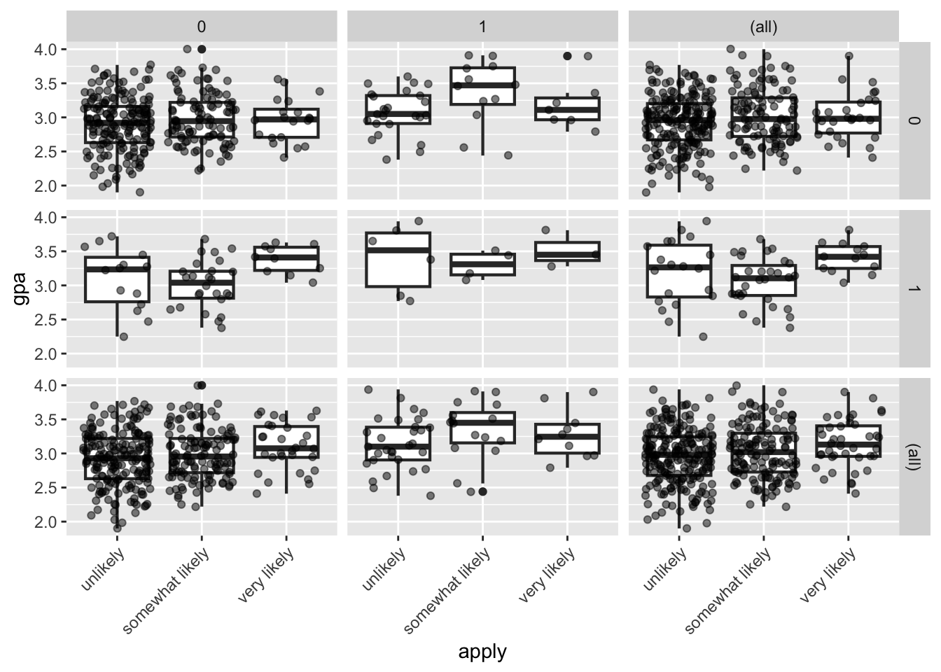

We fit the ordinal logistic regression using the polr() function.

library(MASS)
fit <- polr(apply~pared + public + gpa, data=dat, Hess=TRUE)
summary(fit)

## Call:
## polr(formula = apply ~ pared + public + gpa, data = dat, Hess = TRUE)
## 
## Coefficients:
##           Value Std. Error t value
## pared   1.04769     0.2658  3.9418
## public -0.05879     0.2979 -0.1974
## gpa     0.61594     0.2606  2.3632
## 
## Intercepts:
##                             Value   Std. Error t value
## unlikely|somewhat likely     2.2039  0.7795     2.8272
## somewhat likely|very likely  4.2994  0.8043     5.3453
## 
## Residual Deviance: 717.0249 
## AIC: 727.0249

• For unlikely(1), somewhat likely(2), very likely(3), the estimated model can be written as: $$logit(P(y\leq 1)) = 2.20 -1.05 pared +0.06 public -0.62 gpa$$ $$logit(P(y\leq 2) = 4.30 -1.05 pared +0.06 public -0.62 gpa$$

• There is no p-values. But you know what to do.. The Wald test..

ctable <- coef(summary(fit))
pvals <- pnorm(abs(ctable[,'t value']), lower.tail=F) * 2
ctable <- cbind(ctable,'p value'=pvals)
ci <- confint(fit)

## Waiting for profiling to be done...

cbind(OR=exp(coef(fit)),exp(ci))

##               OR     2.5 %   97.5 %
## pared  2.8510579 1.6958376 4.817114
## public 0.9429088 0.5208954 1.680579
## gpa    1.8513972 1.1136247 3.098490

These are called proportional odds ratios and the interpretation is the same as the binary logistic regression.

DIY Describe the proportional odds assumption in the model. Evaluate whether the model fit is appropriate by testing this assumption. If the assumption is violated, suggest alternative modeling approaches that may provide a better fit.

8.5.1.2 The latent variable interpretation with cutpoints

We easily generalize the probit model formulation for binary outcome to $K$ categories. We assume to observe $y$ by the underlying continuous latent variable $z$: $$y_i = k I(z_i \in (\tau_{k-1},\tau_k)), \textrm{ } k=1,\ldots, K,$$ where $\tau_0=-\infty$, $\tau_1=0$ and $\tau_K = \infty$. $$z_i = X_i\beta + \epsilon_i$$

8.5.2 The unordered model

Multinomial logistic regression is used to model nominal outcome variable.

dat <- read.dta("https://stats.idre.ucla.edu/stat/data/hsbdemo.dta")
head(dat)

##    id female    ses schtyp     prog read write math science socst       honors awards cid
## 1  45 female    low public vocation   34    35   41      29    26 not enrolled      0   1
## 2 108   male middle public  general   34    33   41      36    36 not enrolled      0   1
## 3  15   male   high public vocation   39    39   44      26    42 not enrolled      0   1
## 4  67   male    low public vocation   37    37   42      33    32 not enrolled      0   1
## 5 153   male middle public vocation   39    31   40      39    51 not enrolled      0   1
## 6  51 female   high public  general   42    36   42      31    39 not enrolled      0   1

Entering high school students make program choices among general program, vocational program and academic program. Their choice might be modeled using their writing score and their social economic status. The data set contains variables on 200 students. The outcome variable is prog, program type. The predictor variables are social economic status, ses, a three-level categorical variable and writing score, write, a continuous variable. Let’s start with getting some descriptive statistics of the variables of interest.

with(dat, table(ses, prog))

##         prog
## ses      general academic vocation
##   low         16       19       12
##   middle      20       44       31
##   high         9       42        7

with(dat, do.call(rbind, tapply(write, prog, function(x) c(M = mean(x), SD = sd(x)))))

##                 M       SD
## general  51.33333 9.397775
## academic 56.25714 7.943343
## vocation 46.76000 9.318754

We fit the multinomial model using multinom().

library(nnet)
dat$prog2 <- relevel(dat$prog, ref = "academic")
fit <- multinom(prog2 ~ ses + write, data = dat)

## # weights:  15 (8 variable)
## initial  value 219.722458 
## iter  10 value 179.982880
## final  value 179.981726 
## converged

summary(fit)

## Call:
## multinom(formula = prog2 ~ ses + write, data = dat)
## 
## Coefficients:
##          (Intercept)  sesmiddle    seshigh      write
## general     2.852198 -0.5332810 -1.1628226 -0.0579287
## vocation    5.218260  0.2913859 -0.9826649 -0.1136037
## 
## Std. Errors:
##          (Intercept) sesmiddle   seshigh      write
## general     1.166441 0.4437323 0.5142196 0.02141097
## vocation    1.163552 0.4763739 0.5955665 0.02221996
## 
## Residual Deviance: 359.9635 
## AIC: 375.9635

• The Wald test statistic and p values can be calculated:

z <- summary(fit)$coefficients/summary(fit)$standard.errors
z

##          (Intercept)  sesmiddle   seshigh     write
## general     2.445214 -1.2018081 -2.261334 -2.705562
## vocation    4.484769  0.6116747 -1.649967 -5.112689

p <- (1-pnorm(abs(z)))*2
p

##           (Intercept) sesmiddle    seshigh        write
## general  0.0144766100 0.2294379 0.02373856 6.818902e-03
## vocation 0.0000072993 0.5407530 0.09894976 3.176045e-07

• the model is $$\log\frac{P(prog=general)}{P(prog=academic)} = 2.85 -0.53I(ses=middle) -1.16I(ses=high) -0.061write$$ $$\log\frac{P(prog=vocation)}{P(prog=academic)} = 5.22 +0.29I(ses=middle) -0.98I(ses=high) -0.111write$$

• The ratio of the probability of choosing one outcome category over the probability of choosing the baseline category is often referred as relative risk.

library(tidyverse)