Chapter 6 Lab 4 - 20/10/2022
In this lecture we will learn another R programming approach based on the tidyverse package. This is alternative to the base R code we learnt in the first lectures.
6.1 Tidyverse
Tidyverse is a collection of R packages designed for data science (see Figure 6.1. All the packages share an underlying design philosophy, grammar, and data structures. See here for more details.
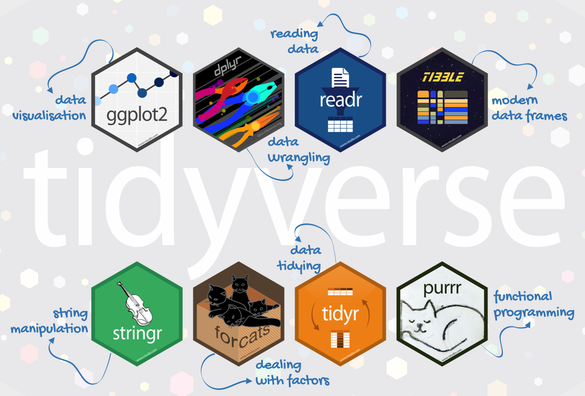
Figure 6.1: Packages included in tidyverse
The tidyverse-based functions process faster than base R
functions. It is because they are written
in a computationally efficient manner and are
also more stable in the syntax and better supports
data frames than vectors.
6.2 Install and load a package
Before starting using a package it is necessary to follow two steps:
install the package: this has to be done only once (unless you re-install R, change or reset your computer). It is like buying a light bulb and installing it in the lamp, as described in Figure 6.2: you do this only once not every time you need some light in your room. This step can be performed by using the RStudio menu, through Tools - Install package, as shown in Figure ??. Behind this menu shortcut RStudio is using the
install.packagesfunction.load the package: this is like switching on the light one you have an installed light bulb, something that can be done every time you need some light in the room (see Figure 6.2). Similarly, each package can be loaded whenever you need to use some functions included in the package. To load the
tidyversepackage we proceed as follows:
library(tidyverse)## ── Attaching packages ─────────────────────────────────────── tidyverse 1.3.2 ──
## ✔ ggplot2 3.3.6 ✔ purrr 0.3.4
## ✔ tibble 3.1.7 ✔ dplyr 1.0.9
## ✔ tidyr 1.2.0 ✔ stringr 1.4.0
## ✔ readr 2.1.2 ✔ forcats 0.5.1
## ── Conflicts ────────────────────────────────────────── tidyverse_conflicts() ──
## ✖ dplyr::filter() masks stats::filter()
## ✖ dplyr::lag() masks stats::lag()
Figure 6.2: Install and load a R package
6.3 The pipe operator
Let’s consider a general R function named f with argument x. We usually
use the following approach when we need to apply f:
f(x)An alternative is given by the pipe operator %>% which is part of the
dplyr package (see here for more details). It works as follows
x %>% f()
#this is equivalent to f(x)
Basically, the pipe tells R to pass x as the first argument of the function f. The shortcut to type the pipe operator in RStudio is given by CTRL/CMD Shift M.
We simulate a sample of data in order to run some simple examples with the pipe operator. By using the function sample we draw randomly (without replacement) 5 numbers between 1 and 20 (1:20).
set.seed(4)
x = sample(1:20, 5)
x
## [1] 11 19 3 7 12We are now interested in computing the log transformation of the vector x. By adopting the standard R programming we would use:
log(x)## [1] 2.397895 2.944439 1.098612 1.945910 2.484907while with the pipe operator we have
x %>% log()## [1] 2.397895 2.944439 1.098612 1.945910 2.484907#it's also possible to omit the parentheses given that there is no inputwhere x is taken as the first argument of the function log. It is also possible to include other arguments, such as for example the base of the logarithm (in this case equal to 5). In this case note that x %>% f(y) is equivalent to f(x,y).
#standard programming
log(x, base=5)
## [1] 1.4898961 1.8294828 0.6826062 1.2090620 1.5439593#pipe based programming
x %>% log(base=5)## [1] 1.4898961 1.8294828 0.6826062 1.2090620 1.5439593We want now to apply the log transformation and then round the corresponding output to 2 digits. This requires the use of two functions (log and round). In general, when we apply 3 functions (f and then g and finally h), we have that x %>% f %>% g %>% h is equivalent to h(g(f(x))).
# standard programming
round(log(x), 2)
## [1] 2.40 2.94 1.10 1.95 2.48# pipe based programming
x %>% log %>% round(2)## [1] 2.40 2.94 1.10 1.95 2.48We now add a new function: after rounding the log output we compute the sum of the 5 numbers
# standard programming
sum(round(log(x),2))
## [1] 10.87# pipe based programming
x %>% log %>% round(2) %>% sum ## [1] 10.87We want now to use the sum result as the base of the log transformation of the number 5
# standard programming
log(5, base = sum(round(log(x),2)))
## [1] 0.674532# pipe based programming
x %>% log %>% round(2) %>% sum %>% log(5,base=.) ## [1] 0.674532The symbol . is the placeholder and is used when the output of the previous pipe should not be used as the first input of the following function. In general, x %>% f(y, z = .) is equivalent to f(y, z = x).
When it is not convenient to use the pipe:
- when the pipes are longer than 10 steps. In this case the suggestion is to create intermediate objects with meaningful names (that can help understanding what the code does);
- when you have multiple inputs or outputs (e.g. when there is no primary object being transformed but two or more objects being combined together).
6.4 dyplyr verbs
dplyr (a package in the tidyverse collection) is a grammar of data manipulation, providing a consistent set of
verbs that help you solve the most common data manipulation challenges:
select: pick variables (columns) based on their namesfilterpick observations (rows) based on their valuesmutate: add new variables that are functions of existing variablessummarise: reduce multiple values down to a single summary (e.g. mean)arrange: change the ordering of the rows
All verbs work similarly:
- the first argument is a data frame;
- the subsequent arguments describe what to do with the data frame using the variable names (without quotes);
- the result is a new data frame.
In the following we will take into account all the dplyr verbs by considering
the diamonds dataset which contains the prices and other attributes of almost 54,000 diamonds (see ?diamonds). If we use the function class to understand the nature of diamonds we get the following output:
class(diamonds)## [1] "tbl_df" "tbl" "data.frame"The term tbl (tibble) is the tidyverse version of a classical R data frame. Tiblles are very similar to data frame (they just contain/display more information) and are designed to be used with the tidyverse syntax style.
To get the list and the type of variables included in diamonds we can use the standard str or the corresponding tidyverse function named glimpse:
str(diamonds)## tibble [53,940 × 10] (S3: tbl_df/tbl/data.frame)
## $ carat : num [1:53940] 0.23 0.21 0.23 0.29 0.31 0.24 0.24 0.26 0.22 0.23 ...
## $ cut : Ord.factor w/ 5 levels "Fair"<"Good"<..: 5 4 2 4 2 3 3 3 1 3 ...
## $ color : Ord.factor w/ 7 levels "D"<"E"<"F"<"G"<..: 2 2 2 6 7 7 6 5 2 5 ...
## $ clarity: Ord.factor w/ 8 levels "I1"<"SI2"<"SI1"<..: 2 3 5 4 2 6 7 3 4 5 ...
## $ depth : num [1:53940] 61.5 59.8 56.9 62.4 63.3 62.8 62.3 61.9 65.1 59.4 ...
## $ table : num [1:53940] 55 61 65 58 58 57 57 55 61 61 ...
## $ price : int [1:53940] 326 326 327 334 335 336 336 337 337 338 ...
## $ x : num [1:53940] 3.95 3.89 4.05 4.2 4.34 3.94 3.95 4.07 3.87 4 ...
## $ y : num [1:53940] 3.98 3.84 4.07 4.23 4.35 3.96 3.98 4.11 3.78 4.05 ...
## $ z : num [1:53940] 2.43 2.31 2.31 2.63 2.75 2.48 2.47 2.53 2.49 2.39 ...glimpse(diamonds)## Rows: 53,940
## Columns: 10
## $ carat <dbl> 0.23, 0.21, 0.23, 0.29, 0.31, 0.24, 0.24, 0.26, 0.22, 0.23, 0.…
## $ cut <ord> Ideal, Premium, Good, Premium, Good, Very Good, Very Good, Ver…
## $ color <ord> E, E, E, I, J, J, I, H, E, H, J, J, F, J, E, E, I, J, J, J, I,…
## $ clarity <ord> SI2, SI1, VS1, VS2, SI2, VVS2, VVS1, SI1, VS2, VS1, SI1, VS1, …
## $ depth <dbl> 61.5, 59.8, 56.9, 62.4, 63.3, 62.8, 62.3, 61.9, 65.1, 59.4, 64…
## $ table <dbl> 55, 61, 65, 58, 58, 57, 57, 55, 61, 61, 55, 56, 61, 54, 62, 58…
## $ price <int> 326, 326, 327, 334, 335, 336, 336, 337, 337, 338, 339, 340, 34…
## $ x <dbl> 3.95, 3.89, 4.05, 4.20, 4.34, 3.94, 3.95, 4.07, 3.87, 4.00, 4.…
## $ y <dbl> 3.98, 3.84, 4.07, 4.23, 4.35, 3.96, 3.98, 4.11, 3.78, 4.05, 4.…
## $ z <dbl> 2.43, 2.31, 2.31, 2.63, 2.75, 2.48, 2.47, 2.53, 2.49, 2.39, 2.…6.4.1 Verb 1: select
This verb is used to select some of the columns by name. For example, to select the variable named carat we use the following code:
diamonds %>% select(carat) ## # A tibble: 53,940 × 1
## carat
## <dbl>
## 1 0.23
## 2 0.21
## 3 0.23
## 4 0.29
## 5 0.31
## 6 0.24
## 7 0.24
## 8 0.26
## 9 0.22
## 10 0.23
## # … with 53,930 more rowsSelecting more than one column is very simple:
diamonds %>% select(carat, cut, color, price)## # A tibble: 53,940 × 4
## carat cut color price
## <dbl> <ord> <ord> <int>
## 1 0.23 Ideal E 326
## 2 0.21 Premium E 326
## 3 0.23 Good E 327
## 4 0.29 Premium I 334
## 5 0.31 Good J 335
## 6 0.24 Very Good J 336
## 7 0.24 Very Good I 336
## 8 0.26 Very Good H 337
## 9 0.22 Fair E 337
## 10 0.23 Very Good H 338
## # … with 53,930 more rowsGiven that carat, cut and color are consecutive, the following code is also possible:
diamonds %>% select(carat : color, price)## # A tibble: 53,940 × 4
## carat cut color price
## <dbl> <ord> <ord> <int>
## 1 0.23 Ideal E 326
## 2 0.21 Premium E 326
## 3 0.23 Good E 327
## 4 0.29 Premium I 334
## 5 0.31 Good J 335
## 6 0.24 Very Good J 336
## 7 0.24 Very Good I 336
## 8 0.26 Very Good H 337
## 9 0.22 Fair E 337
## 10 0.23 Very Good H 338
## # … with 53,930 more rowsMoreover, it is also possible to select all the columns whose name starts with the letter “c” by using starts_with combined with the select function:
diamonds %>% select(starts_with("c"))## # A tibble: 53,940 × 4
## carat cut color clarity
## <dbl> <ord> <ord> <ord>
## 1 0.23 Ideal E SI2
## 2 0.21 Premium E SI1
## 3 0.23 Good E VS1
## 4 0.29 Premium I VS2
## 5 0.31 Good J SI2
## 6 0.24 Very Good J VVS2
## 7 0.24 Very Good I VVS1
## 8 0.26 Very Good H SI1
## 9 0.22 Fair E VS2
## 10 0.23 Very Good H VS1
## # … with 53,930 more rowsIt is also possible to specify a criterion which excludes from the selection some variables. For example, to select all the columns but carat we use the - symbol:
diamonds %>% select(-carat)## # A tibble: 53,940 × 9
## cut color clarity depth table price x y z
## <ord> <ord> <ord> <dbl> <dbl> <int> <dbl> <dbl> <dbl>
## 1 Ideal E SI2 61.5 55 326 3.95 3.98 2.43
## 2 Premium E SI1 59.8 61 326 3.89 3.84 2.31
## 3 Good E VS1 56.9 65 327 4.05 4.07 2.31
## 4 Premium I VS2 62.4 58 334 4.2 4.23 2.63
## 5 Good J SI2 63.3 58 335 4.34 4.35 2.75
## 6 Very Good J VVS2 62.8 57 336 3.94 3.96 2.48
## 7 Very Good I VVS1 62.3 57 336 3.95 3.98 2.47
## 8 Very Good H SI1 61.9 55 337 4.07 4.11 2.53
## 9 Fair E VS2 65.1 61 337 3.87 3.78 2.49
## 10 Very Good H VS1 59.4 61 338 4 4.05 2.39
## # … with 53,930 more rowsWe proceed similarly to select all the columns but not the ones with a name starting with “c”:
diamonds %>% select(- starts_with("c"))## # A tibble: 53,940 × 6
## depth table price x y z
## <dbl> <dbl> <int> <dbl> <dbl> <dbl>
## 1 61.5 55 326 3.95 3.98 2.43
## 2 59.8 61 326 3.89 3.84 2.31
## 3 56.9 65 327 4.05 4.07 2.31
## 4 62.4 58 334 4.2 4.23 2.63
## 5 63.3 58 335 4.34 4.35 2.75
## 6 62.8 57 336 3.94 3.96 2.48
## 7 62.3 57 336 3.95 3.98 2.47
## 8 61.9 55 337 4.07 4.11 2.53
## 9 65.1 61 337 3.87 3.78 2.49
## 10 59.4 61 338 4 4.05 2.39
## # … with 53,930 more rowsAnother useful application is the selection of only the numerical variables. This can be performed by using the select_if function combined with is.numeric (the latter is a test of an object being interpretable as numbers):
diamonds %>%
  select_if(is.numeric)
## # A tibble: 53,940 × 7
## carat depth table price x y z
## <dbl> <dbl> <dbl> <int> <dbl> <dbl> <dbl>
## 1 0.23 61.5 55 326 3.95 3.98 2.43
## 2 0.21 59.8 61 326 3.89 3.84 2.31
## 3 0.23 56.9 65 327 4.05 4.07 2.31
## 4 0.29 62.4 58 334 4.2 4.23 2.63
## 5 0.31 63.3 58 335 4.34 4.35 2.75
## 6 0.24 62.8 57 336 3.94 3.96 2.48
## 7 0.24 62.3 57 336 3.95 3.98 2.47
## 8 0.26 61.9 55 337 4.07 4.11 2.53
## 9 0.22 65.1 61 337 3.87 3.78 2.49
## 10 0.23 59.4 61 338 4 4.05 2.39
## # … with 53,930 more rowsThe returned output can be then used to compute jointly all the averages of the numerical variables by using the apply function (see ??):
diamonds %>%
  select_if(is.numeric) %>%
  apply(2, mean)
## carat depth table price x y
## 0.7979397 61.7494049 57.4571839 3932.7997219 5.7311572 5.7345260
## z
## 3.53873386.4.2 Verb 2: filter
The verb filter can be used to select the observations satisfying some criterion. Consider the example the selection of the diamonds with variable cut equal to the category “Premium”:
diamonds %>% filter(cut == "Premium")## # A tibble: 13,791 × 10
## carat cut color clarity depth table price x y z
## <dbl> <ord> <ord> <ord> <dbl> <dbl> <int> <dbl> <dbl> <dbl>
## 1 0.21 Premium E SI1 59.8 61 326 3.89 3.84 2.31
## 2 0.29 Premium I VS2 62.4 58 334 4.2 4.23 2.63
## 3 0.22 Premium F SI1 60.4 61 342 3.88 3.84 2.33
## 4 0.2 Premium E SI2 60.2 62 345 3.79 3.75 2.27
## 5 0.32 Premium E I1 60.9 58 345 4.38 4.42 2.68
## 6 0.24 Premium I VS1 62.5 57 355 3.97 3.94 2.47
## 7 0.29 Premium F SI1 62.4 58 403 4.24 4.26 2.65
## 8 0.22 Premium E VS2 61.6 58 404 3.93 3.89 2.41
## 9 0.22 Premium D VS2 59.3 62 404 3.91 3.88 2.31
## 10 0.3 Premium J SI2 59.3 61 405 4.43 4.38 2.61
## # … with 13,781 more rowsIt is also possible to include more conditions. Select for example the diamonds with cut equal to “Premium” AND color equal to “D” (the AND can be specified by using & or comma):
diamonds %>% filter(cut == "Premium" & color == "D") ## # A tibble: 1,603 × 10
## carat cut color clarity depth table price x y z
## <dbl> <ord> <ord> <ord> <dbl> <dbl> <int> <dbl> <dbl> <dbl>
## 1 0.22 Premium D VS2 59.3 62 404 3.91 3.88 2.31
## 2 0.3 Premium D SI1 62.6 59 552 4.23 4.27 2.66
## 3 0.71 Premium D SI2 61.7 59 2768 5.71 5.67 3.51
## 4 0.71 Premium D VS2 62.5 60 2770 5.65 5.61 3.52
## 5 0.7 Premium D VS2 58 62 2773 5.87 5.78 3.38
## 6 0.72 Premium D SI1 62.7 59 2782 5.73 5.69 3.58
## 7 0.7 Premium D SI1 62.8 60 2782 5.68 5.66 3.56
## 8 0.72 Premium D SI2 62 60 2795 5.73 5.69 3.54
## 9 0.71 Premium D SI1 62.7 60 2797 5.67 5.71 3.57
## 10 0.71 Premium D SI1 61.3 58 2797 5.73 5.75 3.52
## # … with 1,593 more rowsdiamonds %>% filter(cut == "Premium" , color == "D") ## # A tibble: 1,603 × 10
## carat cut color clarity depth table price x y z
## <dbl> <ord> <ord> <ord> <dbl> <dbl> <int> <dbl> <dbl> <dbl>
## 1 0.22 Premium D VS2 59.3 62 404 3.91 3.88 2.31
## 2 0.3 Premium D SI1 62.6 59 552 4.23 4.27 2.66
## 3 0.71 Premium D SI2 61.7 59 2768 5.71 5.67 3.51
## 4 0.71 Premium D VS2 62.5 60 2770 5.65 5.61 3.52
## 5 0.7 Premium D VS2 58 62 2773 5.87 5.78 3.38
## 6 0.72 Premium D SI1 62.7 59 2782 5.73 5.69 3.58
## 7 0.7 Premium D SI1 62.8 60 2782 5.68 5.66 3.56
## 8 0.72 Premium D SI2 62 60 2795 5.73 5.69 3.54
## 9 0.71 Premium D SI1 62.7 60 2797 5.67 5.71 3.57
## 10 0.71 Premium D SI1 61.3 58 2797 5.73 5.75 3.52
## # … with 1,593 more rowsIf we are interested in filtering th diamonds with a price between 500 and 600 dollars the following two alternative codes can be adopted:
diamonds %>% filter(price > 500 & price < 600)## # A tibble: 2,360 × 10
## carat cut color clarity depth table price x y z
## <dbl> <ord> <ord> <ord> <dbl> <dbl> <int> <dbl> <dbl> <dbl>
## 1 0.35 Ideal I VS1 60.9 57 552 4.54 4.59 2.78
## 2 0.3 Premium D SI1 62.6 59 552 4.23 4.27 2.66
## 3 0.3 Ideal D SI1 62.5 57 552 4.29 4.32 2.69
## 4 0.3 Ideal D SI1 62.1 56 552 4.3 4.33 2.68
## 5 0.42 Premium I SI2 61.5 59 552 4.78 4.84 2.96
## 6 0.28 Ideal G VVS2 61.4 56 553 4.19 4.22 2.58
## 7 0.32 Ideal I VVS1 62 55.3 553 4.39 4.42 2.73
## 8 0.31 Very Good G SI1 63.3 57 553 4.33 4.3 2.73
## 9 0.31 Premium G SI1 61.8 58 553 4.35 4.32 2.68
## 10 0.24 Premium E VVS1 60.7 58 553 4.01 4.03 2.44
## # … with 2,350 more rowsdiamonds %>% filter(between(price, 500,600))## # A tibble: 2,407 × 10
## carat cut color clarity depth table price x y z
## <dbl> <ord> <ord> <ord> <dbl> <dbl> <int> <dbl> <dbl> <dbl>
## 1 0.35 Ideal I VS1 60.9 57 552 4.54 4.59 2.78
## 2 0.3 Premium D SI1 62.6 59 552 4.23 4.27 2.66
## 3 0.3 Ideal D SI1 62.5 57 552 4.29 4.32 2.69
## 4 0.3 Ideal D SI1 62.1 56 552 4.3 4.33 2.68
## 5 0.42 Premium I SI2 61.5 59 552 4.78 4.84 2.96
## 6 0.28 Ideal G VVS2 61.4 56 553 4.19 4.22 2.58
## 7 0.32 Ideal I VVS1 62 55.3 553 4.39 4.42 2.73
## 8 0.31 Very Good G SI1 63.3 57 553 4.33 4.3 2.73
## 9 0.31 Premium G SI1 61.8 58 553 4.35 4.32 2.68
## 10 0.24 Premium E VVS1 60.7 58 553 4.01 4.03 2.44
## # … with 2,397 more rowsThe output of a selection can always be saved in a new data frame as follows:
out = diamonds %>% filter(between(price, 500,600))To select diamonds with cut equal to fair OR good we can use the | operator or the %in% function:
diamonds %>% filter(cut=="Fair" | cut=="Good")## # A tibble: 6,516 × 10
## carat cut color clarity depth table price x y z
## <dbl> <ord> <ord> <ord> <dbl> <dbl> <int> <dbl> <dbl> <dbl>
## 1 0.23 Good E VS1 56.9 65 327 4.05 4.07 2.31
## 2 0.31 Good J SI2 63.3 58 335 4.34 4.35 2.75
## 3 0.22 Fair E VS2 65.1 61 337 3.87 3.78 2.49
## 4 0.3 Good J SI1 64 55 339 4.25 4.28 2.73
## 5 0.3 Good J SI1 63.4 54 351 4.23 4.29 2.7
## 6 0.3 Good J SI1 63.8 56 351 4.23 4.26 2.71
## 7 0.3 Good I SI2 63.3 56 351 4.26 4.3 2.71
## 8 0.23 Good F VS1 58.2 59 402 4.06 4.08 2.37
## 9 0.23 Good E VS1 64.1 59 402 3.83 3.85 2.46
## 10 0.31 Good H SI1 64 54 402 4.29 4.31 2.75
## # … with 6,506 more rowsdiamonds %>% filter(cut %in% c("Fair","Good"))## # A tibble: 6,516 × 10
## carat cut color clarity depth table price x y z
## <dbl> <ord> <ord> <ord> <dbl> <dbl> <int> <dbl> <dbl> <dbl>
## 1 0.23 Good E VS1 56.9 65 327 4.05 4.07 2.31
## 2 0.31 Good J SI2 63.3 58 335 4.34 4.35 2.75
## 3 0.22 Fair E VS2 65.1 61 337 3.87 3.78 2.49
## 4 0.3 Good J SI1 64 55 339 4.25 4.28 2.73
## 5 0.3 Good J SI1 63.4 54 351 4.23 4.29 2.7
## 6 0.3 Good J SI1 63.8 56 351 4.23 4.26 2.71
## 7 0.3 Good I SI2 63.3 56 351 4.26 4.3 2.71
## 8 0.23 Good F VS1 58.2 59 402 4.06 4.08 2.37
## 9 0.23 Good E VS1 64.1 59 402 3.83 3.85 2.46
## 10 0.31 Good H SI1 64 54 402 4.29 4.31 2.75
## # … with 6,506 more rowsThe code diamonds %>% filter(cut == c("Fair","Good")) does not perform what we mean to do. For an interesting discussion about the difference between == and %in% see here.
6.4.3 Verb 4: summarise
This verbs can be used to compute summary statistics. For example the following code computes the mean and median of price.
diamonds %>%
  summarise(mean(price),
            median(price))
## # A tibble: 1 × 2
## `mean(price)` `median(price)`
## <dbl> <dbl>
## 1 3933. 2401The output is automatically labelled but it is also possible to specify different labels as follows:
diamonds %>%
  summarise(mean_price = mean(price),
            median_price = median(price))
## # A tibble: 1 × 2
## mean_price median_price
## <dbl> <dbl>
## 1 3933. 2401Similarly, it is possible to compute some summary statistics on a new variable which is a transformation of the variables originally contained in the data frame. For example, we are interested in the mean of a new variable given by the price per unit given by the ration between price and carat:
diamonds %>%
  summarise(mean_unitprice = mean(price/carat))
## # A tibble: 1 × 1
## mean_unitprice
## <dbl>
## 1 4008.Another transformation of the original variables consists in considering if a price is bigger than 1000$ (T or F) and then computing how many observations (absolute frequency, proportion or percentage) satisfy the condition. This is computed by using the sum or mean functions:
diamonds %>%
  summarise(veryexp = sum(price > 1000),
            veryexpprop = mean(price>1000),
            veryexpperc = mean(price>1000)*100)
## # A tibble: 1 × 3
## veryexp veryexpprop veryexpperc
## <int> <dbl> <dbl>
## 1 39416 0.731 73.1It is also interesting to compute summary statistics conditionally on the categories of a qualitative variable (i.e. a factor). This can be done by combining the group_by function with the summarise function. Let’s compute for example the mean, min and max price conditionally on the categories of cut:
diamonds %>%
  group_by(cut) %>%
  summarise(mean(price),min(price),max(price))
## # A tibble: 5 × 4
## cut `mean(price)` `min(price)` `max(price)`
## <ord> <dbl> <int> <int>
## 1 Fair 4359. 337 18574
## 2 Good 3929. 327 18788
## 3 Very Good 3982. 336 18818
## 4 Premium 4584. 326 18823
## 5 Ideal 3458. 326 18806In particular, group_by splits the original data set into different groups (according to the category of the group_by variable) and for each of them the requested summary statistics are computed. In this case we obtain 5 values of the mean, min and max price according to the number of categories of the variable cut. It is also possible to condition on two different factors, such as for example cut and color:
diamonds %>%
  group_by(cut,color) %>%
  summarise(mean(price))
## `summarise()` has grouped output by 'cut'. You can override using the `.groups`
## argument.## # A tibble: 35 × 3
## # Groups: cut [5]
## cut color `mean(price)`
## <ord> <ord> <dbl>
## 1 Fair D 4291.
## 2 Fair E 3682.
## 3 Fair F 3827.
## 4 Fair G 4239.
## 5 Fair H 5136.
## 6 Fair I 4685.
## 7 Fair J 4976.
## 8 Good D 3405.
## 9 Good E 3424.
## 10 Good F 3496.
## # … with 25 more rowsIn this case each category of cut is combined with each category of color and then the mean price is computed.
The function group_by can by combined with summarise also to compute frequency distribution, by means of the n() function which gives the current group size:
diamonds %>%
  group_by(cut) %>%
  summarise(AbsFreq = n())
## # A tibble: 5 × 2
## cut AbsFreq
## <ord> <int>
## 1 Fair 1610
## 2 Good 4906
## 3 Very Good 12082
## 4 Premium 13791
## 5 Ideal 21551This is an alternative to the table standard function:
table(diamonds$cut)##
## Fair Good Very Good Premium Ideal
## 1610 4906 12082 13791 21551Similarly, percentages can be easily computed by using AbsFreq represents a new variable available for new computations:
diamonds %>%
  group_by(cut) %>%
  summarise(AbsFreq = n(),
            Perc = AbsFreq/nrow(diamonds)*100)
## # A tibble: 5 × 3
## cut AbsFreq Perc
## <ord> <int> <dbl>
## 1 Fair 1610 2.98
## 2 Good 4906 9.10
## 3 Very Good 12082 22.4
## 4 Premium 13791 25.6
## 5 Ideal 21551 40.0A shorter alternative for computing the frequency table si given by the count function which let you quickly count the unique values of one or more variables. Basically, df %>% count(a, b) is roughly equivalent to df %>% group_by(a, b) %>% summarise(n = n()). Here below we have an example:
diamonds %>%
  count(cut)
## # A tibble: 5 × 2
## cut n
## <ord> <int>
## 1 Fair 1610
## 2 Good 4906
## 3 Very Good 12082
## 4 Premium 13791
## 5 Ideal 215516.5 Exercises Lecture 4
6.5.1 Exercise 1
Write the code for the following operations:
- Simulate a vector of 15 values from the continuous Uniform distribution defined between 0 and 10 (see
?runif). Set the seed equal to 99. - Round the numbers in the vector to two digits.
- Sort the values in the vector in descending order (see
?sort) - Display a few of the largest values with
head().
Use both the standard R programming approach and the more modern approach based on the use of the pipe %>% (remember to load the tidyverse library).
6.5.2 Exercise 2
Consider the mtcars data set which is available in R. Type the following code to explore the variables included in the data set (for an explanation of the variables see ?mtcars:
library(tidyverse)
glimpse(mtcars)
## Rows: 32
## Columns: 11
## $ mpg <dbl> 21.0, 21.0, 22.8, 21.4, 18.7, 18.1, 14.3, 24.4, 22.8, 19.2, 17.8,…
## $ cyl <dbl> 6, 6, 4, 6, 8, 6, 8, 4, 4, 6, 6, 8, 8, 8, 8, 8, 8, 4, 4, 4, 4, 8,…
## $ disp <dbl> 160.0, 160.0, 108.0, 258.0, 360.0, 225.0, 360.0, 146.7, 140.8, 16…
## $ hp <dbl> 110, 110, 93, 110, 175, 105, 245, 62, 95, 123, 123, 180, 180, 180…
## $ drat <dbl> 3.90, 3.90, 3.85, 3.08, 3.15, 2.76, 3.21, 3.69, 3.92, 3.92, 3.92,…
## $ wt <dbl> 2.620, 2.875, 2.320, 3.215, 3.440, 3.460, 3.570, 3.190, 3.150, 3.…
## $ qsec <dbl> 16.46, 17.02, 18.61, 19.44, 17.02, 20.22, 15.84, 20.00, 22.90, 18…
## $ vs <dbl> 0, 0, 1, 1, 0, 1, 0, 1, 1, 1, 1, 0, 0, 0, 0, 0, 0, 1, 1, 1, 1, 0,…
## $ am <dbl> 1, 1, 1, 0, 0, 0, 0, 0, 0, 0, 0, 0, 0, 0, 0, 0, 0, 1, 1, 1, 0, 0,…
## $ gear <dbl> 4, 4, 4, 3, 3, 3, 3, 4, 4, 4, 4, 3, 3, 3, 3, 3, 3, 4, 4, 4, 3, 3,…
## $ carb <dbl> 4, 4, 1, 1, 2, 1, 4, 2, 2, 4, 4, 3, 3, 3, 4, 4, 4, 1, 2, 1, 1, 2,…Use the following code to create a new variable named car_model that contains the names of the cars, now available as row names.
mtcars = mtcars %>%
        rownames_to_column("car_model")
glimpse(mtcars)
## Rows: 32
## Columns: 12
## $ car_model <chr> "Mazda RX4", "Mazda RX4 Wag", "Datsun 710", "Hornet 4 Drive"…
## $ mpg <dbl> 21.0, 21.0, 22.8, 21.4, 18.7, 18.1, 14.3, 24.4, 22.8, 19.2, …
## $ cyl <dbl> 6, 6, 4, 6, 8, 6, 8, 4, 4, 6, 6, 8, 8, 8, 8, 8, 8, 4, 4, 4, …
## $ disp <dbl> 160.0, 160.0, 108.0, 258.0, 360.0, 225.0, 360.0, 146.7, 140.…
## $ hp <dbl> 110, 110, 93, 110, 175, 105, 245, 62, 95, 123, 123, 180, 180…
## $ drat <dbl> 3.90, 3.90, 3.85, 3.08, 3.15, 2.76, 3.21, 3.69, 3.92, 3.92, …
## $ wt <dbl> 2.620, 2.875, 2.320, 3.215, 3.440, 3.460, 3.570, 3.190, 3.15…
## $ qsec <dbl> 16.46, 17.02, 18.61, 19.44, 17.02, 20.22, 15.84, 20.00, 22.9…
## $ vs <dbl> 0, 0, 1, 1, 0, 1, 0, 1, 1, 1, 1, 0, 0, 0, 0, 0, 0, 1, 1, 1, …
## $ am <dbl> 1, 1, 1, 0, 0, 0, 0, 0, 0, 0, 0, 0, 0, 0, 0, 0, 0, 1, 1, 1, …
## $ gear <dbl> 4, 4, 4, 3, 3, 3, 3, 4, 4, 4, 4, 3, 3, 3, 3, 3, 3, 4, 4, 4, …
## $ carb <dbl> 4, 4, 1, 1, 2, 1, 4, 2, 2, 4, 4, 3, 3, 3, 4, 4, 4, 1, 2, 1, …The variables
cylandamare considered as numerical variable (dbl). Transform them into two factors (decide if you want to set labels):How many observations and variables are available?
Print (on the screen) the
hpvariable using theselect()function. Try also to use thepull()function. Which is the difference?Print out all but the
hpcolumn using theselect()function.Print out the following variables:
mpg,hp,vs,am,gear. Suggestion: use:if necessary.Provide the frequency distribution (absolute, relative and percentage) for the
amvariable (transmission).Select all the observations which have
mpg>20andhp>100and compute the average for thempgvariable.Compute the distribution (absolute frequencies) of the car by
gear. Moreover, compute the mean consumption (mpg) conditionally on thegear.
6.5.3 Exercise 3
Consider the iris dataset available in R. It contains the measurements in centimeters of the variables sepal length and width and petal length and width, respectively, for some flowers from each of 3 species of iris. See ?iris.
glimpse(iris)## Rows: 150
## Columns: 5
## $ Sepal.Length <dbl> 5.1, 4.9, 4.7, 4.6, 5.0, 5.4, 4.6, 5.0, 4.4, 4.9, 5.4, 4.…
## $ Sepal.Width <dbl> 3.5, 3.0, 3.2, 3.1, 3.6, 3.9, 3.4, 3.4, 2.9, 3.1, 3.7, 3.…
## $ Petal.Length <dbl> 1.4, 1.4, 1.3, 1.5, 1.4, 1.7, 1.4, 1.5, 1.4, 1.5, 1.5, 1.…
## $ Petal.Width <dbl> 0.2, 0.2, 0.2, 0.2, 0.2, 0.4, 0.3, 0.2, 0.2, 0.1, 0.2, 0.…
## $ Species <fct> setosa, setosa, setosa, setosa, setosa, setosa, setosa, s…Compute the frequency distribution (absolute, relative and percentage frequencies) of
Species. Which are the available species?Compute the average and the standard deviation for all the numeric column of
iris. Then compute the same statistics by conditioning on species. Suggestion: use the functionsummarise_if(see?summarise_if, in this case test if the columnis.numeric):Compute the average of
Sepal.LengthandPetal.LengthbySpecies. Which is the species with the highest average sepal/petal length?