Chapter 4 Lab 2 - 06/10/2022
In this lecture we will work with different R object.
4.1 (Pseudo) Random number simulation
In Section 3.2 we have already introduced the concept of numerical vector. We will now create a vector containing 10 numbers simulated from the continuous Uniform distribution (see here).
An example of random generation is given by the random experiment that consists in tossing a coin four times (T=tail, H=head). One possible outcome is {T, H, H, T, T}, while {H, H, H, T, H} is another possible random sequence. All the random sequence of Head and Tail are simulated from the distribution which assigns probability 0.5 to Head and probability 0.5 to Tail.
The function sample can be used to perform the coin random experiment (see ?sample). With the following code we toss the coin 10 time (two possible outcomes: head and tail) and save the (random) output in a vector named x which is a vector of strings (character):
x = sample(x = c("head", "tail"), size = 10, replace = TRUE)
class(x) #information about the object
## [1] "character"As the procedure is random every time you run sample you will get a different output.
Given the vector x it is possible to compute how many times we got head/tail and to plot this frequency distribution:
table(x) # frequency distribution ## x
## head tail
## 5 5barplot(table(x)) #plot the frequency distribution 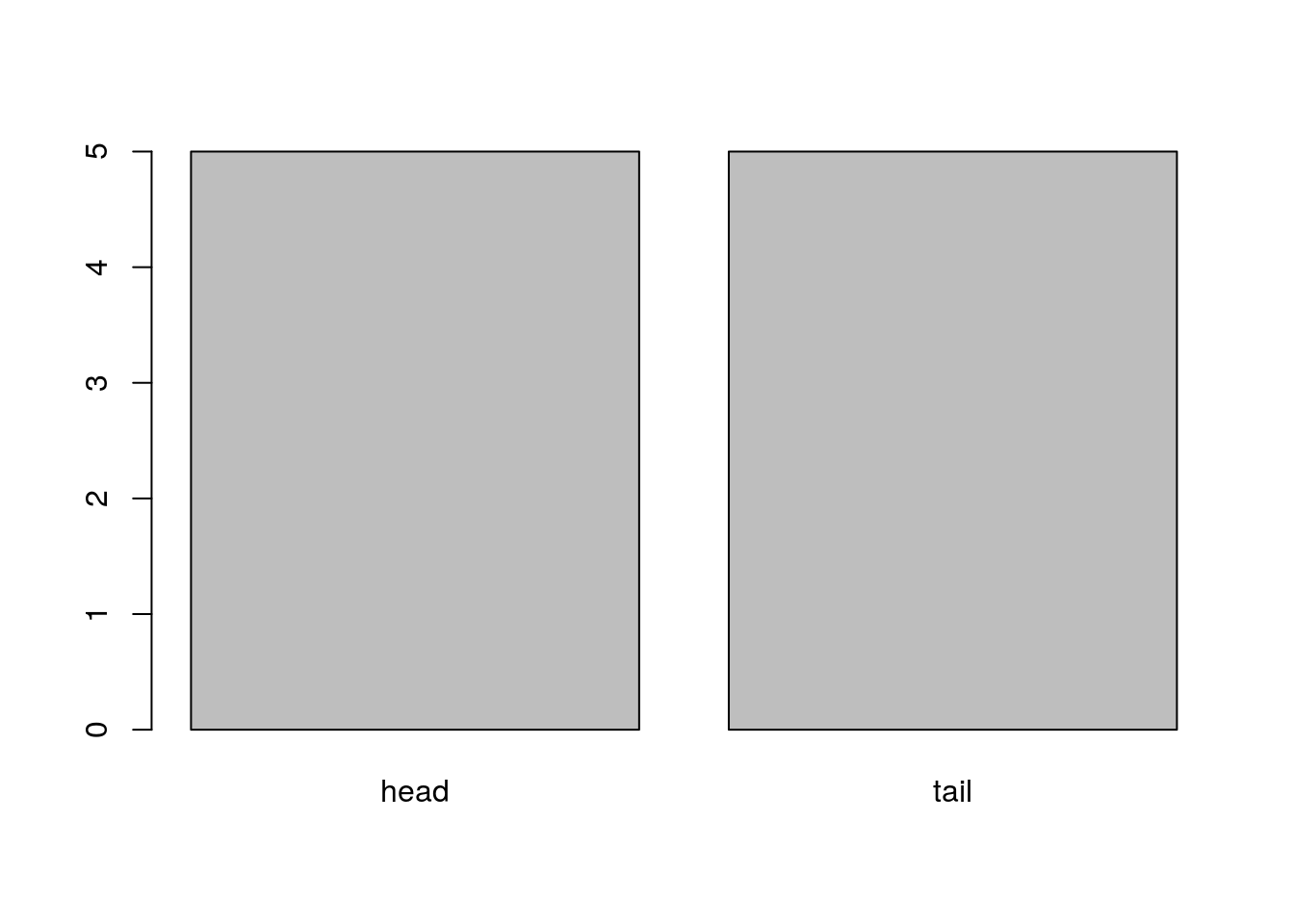
We will proceed similarly by simulating values from the Uniform(0,1) distribution which can take all the real values between 0 and 1. In this case we resort to a specific R function named runif (r... stands for random), see ?runif. For simulating randomly 10 numbers from the Uniform distribution defined with 0 and 1 (default values), we use the following code:
runif(10)## [1] 0.84324669 0.77474887 0.38719298 0.13576507 0.90035758 0.56645266
## [7] 0.04273416 0.48831925 0.35122322 0.96966171This code returns 10 different number every time you run it. In order to get the same data, for reproducibility purposes, it is necessary to set the seed (i.e. to set the starting point of the algorithm which generates the random numbers). To do this the set.seed function is used; it takes as input an integer positive number (55 in the following example):
set.seed(55)
y = runif(10)
y
## [1] 0.54781352 0.21815968 0.03496399 0.79154929 0.56024208 0.07422517
## [7] 0.13152294 0.29412388 0.50076126 0.08832446class(y)## [1] "numeric"The 10 numbers are saved in an object named y which is a numerical vector. By setting the seed we are able to reproduce always the same sequence of random numbers (which is the same for all of us). In this case the numbers are said to be pseudo-random (and not fully random as they can be reproduced).
The 10 values can be plotted by using the following code that returns an histogram:
hist(y)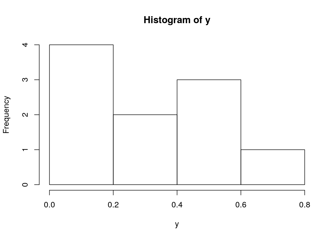
It is also possible to reduce the number of decimals by using the function round (see ?round). For example, we decide to have the number in x with 2 decimals:
z = round(y, 2)
z
## [1] 0.55 0.22 0.03 0.79 0.56 0.07 0.13 0.29 0.50 0.09To check the type of object the function class can be used:
class(z) ## [1] "numeric"In this case z is a vector of real numbers (numeric).
Let’s assume now to combine x and y by concatenating (with the c function) the two vectors:
w = c(x, y)
w
## [1] "tail" "tail" "tail"
## [4] "head" "head" "head"
## [7] "tail" "head" "head"
## [10] "tail" "0.547813516110182" "0.218159678624943"
## [13] "0.0349639947526157" "0.791549294022843" "0.560242076171562"
## [16] "0.0742251740302891" "0.131522935815156" "0.294123877771199"
## [19] "0.500761263305321" "0.088324457872659"class(w)## [1] "character"Note that w is a vector of text strings (character) and also the numbers have been forced to text. This is not happenig if we combine two numerical vectors as y and z:
p = c(y, z)
class(p)
## [1] "numeric"length(p) #check how many elements in p## [1] 204.2 Normal distribution
The Normal distribution is the most known and used continuous random variable (see here). The function for simulating values from the Normal distribution is rnorm (see ?rnorm).
We sample here below 1000 values from the Normal distribution with mean 5 and variance 4.
set.seed(55)
mynorm = rnorm(1000, mean = 5, sd = sqrt(4))
We then plot the simulated data and compute some (empirical) summary statistics:
hist(mynorm)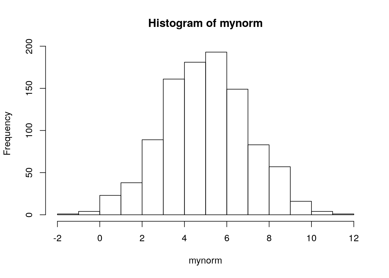
mean(mynorm) #empirical mean## [1] 5.028065var(mynorm) #empirical variance## [1] 4.025442range(mynorm) #min, max## [1] -1.14358 11.95355head(mynorm) #first 6 elements of the vector## [1] 5.240278 1.375246 5.303166 2.761558 5.003816 7.377037We know assume that the 1000 values are scores from a test taken by 1000 students. We want know to compute the number of students who got a score bigger than 6. First of all we check the considered condition which returns a logical vector (remember that TRUE = 1, FALSE = 0):
mynorm > 6 # logical vector ## [1] FALSE FALSE FALSE FALSE FALSE TRUE FALSE FALSE FALSE FALSE FALSE FALSE
## [13] FALSE FALSE FALSE FALSE TRUE TRUE FALSE TRUE FALSE TRUE TRUE TRUE
## [25] TRUE TRUE FALSE TRUE FALSE FALSE TRUE FALSE FALSE FALSE FALSE FALSE
## [37] FALSE FALSE FALSE TRUE TRUE FALSE FALSE TRUE TRUE TRUE FALSE FALSE
## [49] FALSE FALSE FALSE FALSE FALSE FALSE FALSE FALSE TRUE FALSE FALSE FALSE
## [61] TRUE FALSE TRUE TRUE FALSE FALSE TRUE FALSE FALSE FALSE FALSE FALSE
## [73] FALSE FALSE FALSE FALSE FALSE TRUE TRUE FALSE FALSE FALSE FALSE FALSE
## [85] TRUE FALSE FALSE TRUE TRUE FALSE FALSE FALSE FALSE FALSE FALSE FALSE
## [97] FALSE TRUE FALSE TRUE FALSE FALSE FALSE TRUE FALSE TRUE FALSE TRUE
## [109] FALSE TRUE FALSE TRUE TRUE FALSE FALSE TRUE FALSE FALSE TRUE FALSE
## [121] FALSE FALSE TRUE FALSE FALSE FALSE TRUE FALSE FALSE TRUE FALSE TRUE
## [133] TRUE FALSE FALSE FALSE FALSE FALSE FALSE FALSE FALSE FALSE FALSE FALSE
## [145] FALSE TRUE TRUE FALSE FALSE FALSE FALSE FALSE TRUE FALSE FALSE FALSE
## [157] TRUE FALSE FALSE TRUE FALSE TRUE FALSE FALSE FALSE FALSE FALSE FALSE
## [169] TRUE FALSE FALSE FALSE FALSE FALSE FALSE FALSE TRUE FALSE FALSE TRUE
## [181] FALSE TRUE FALSE FALSE FALSE TRUE TRUE FALSE FALSE TRUE TRUE FALSE
## [193] FALSE FALSE FALSE FALSE TRUE TRUE TRUE FALSE FALSE TRUE TRUE FALSE
## [205] TRUE TRUE TRUE FALSE FALSE FALSE FALSE TRUE FALSE TRUE TRUE FALSE
## [217] FALSE TRUE FALSE FALSE FALSE FALSE TRUE FALSE TRUE FALSE FALSE FALSE
## [229] FALSE TRUE FALSE FALSE FALSE FALSE FALSE FALSE FALSE FALSE FALSE FALSE
## [241] TRUE FALSE FALSE FALSE FALSE TRUE TRUE TRUE FALSE TRUE FALSE FALSE
## [253] FALSE FALSE FALSE TRUE FALSE TRUE TRUE FALSE FALSE TRUE TRUE TRUE
## [265] FALSE FALSE FALSE TRUE FALSE FALSE TRUE TRUE FALSE TRUE TRUE TRUE
## [277] FALSE FALSE FALSE TRUE TRUE FALSE FALSE FALSE FALSE FALSE FALSE TRUE
## [289] TRUE TRUE FALSE TRUE FALSE FALSE FALSE TRUE FALSE FALSE FALSE FALSE
## [301] FALSE FALSE FALSE FALSE FALSE TRUE FALSE TRUE FALSE FALSE FALSE TRUE
## [313] FALSE TRUE FALSE FALSE FALSE TRUE FALSE FALSE TRUE FALSE TRUE TRUE
## [325] FALSE TRUE TRUE FALSE FALSE FALSE FALSE FALSE FALSE FALSE TRUE FALSE
## [337] FALSE FALSE TRUE FALSE FALSE FALSE TRUE FALSE FALSE FALSE TRUE FALSE
## [349] FALSE FALSE FALSE FALSE TRUE FALSE FALSE TRUE FALSE TRUE TRUE FALSE
## [361] TRUE FALSE FALSE FALSE FALSE FALSE FALSE FALSE FALSE FALSE FALSE FALSE
## [373] FALSE FALSE FALSE TRUE FALSE FALSE TRUE FALSE FALSE TRUE FALSE FALSE
## [385] FALSE FALSE FALSE FALSE FALSE FALSE FALSE TRUE FALSE FALSE TRUE TRUE
## [397] FALSE FALSE TRUE FALSE TRUE TRUE FALSE TRUE FALSE FALSE FALSE TRUE
## [409] TRUE TRUE FALSE FALSE FALSE FALSE FALSE TRUE FALSE TRUE TRUE FALSE
## [421] FALSE FALSE FALSE TRUE FALSE FALSE FALSE TRUE FALSE FALSE FALSE FALSE
## [433] FALSE FALSE FALSE TRUE TRUE TRUE TRUE FALSE FALSE FALSE FALSE FALSE
## [445] FALSE FALSE FALSE FALSE TRUE FALSE TRUE FALSE FALSE FALSE FALSE FALSE
## [457] FALSE TRUE FALSE FALSE FALSE FALSE FALSE FALSE TRUE FALSE FALSE TRUE
## [469] TRUE FALSE FALSE FALSE FALSE FALSE TRUE FALSE FALSE FALSE FALSE FALSE
## [481] TRUE FALSE FALSE FALSE FALSE FALSE FALSE FALSE FALSE TRUE FALSE FALSE
## [493] TRUE TRUE FALSE FALSE FALSE FALSE FALSE TRUE FALSE FALSE FALSE FALSE
## [505] FALSE FALSE FALSE FALSE TRUE FALSE FALSE TRUE FALSE TRUE FALSE FALSE
## [517] FALSE FALSE FALSE TRUE FALSE FALSE FALSE TRUE FALSE TRUE TRUE FALSE
## [529] FALSE FALSE FALSE FALSE FALSE FALSE TRUE FALSE FALSE TRUE TRUE FALSE
## [541] FALSE TRUE TRUE TRUE FALSE TRUE FALSE FALSE FALSE FALSE FALSE FALSE
## [553] FALSE FALSE FALSE FALSE FALSE FALSE FALSE TRUE FALSE FALSE FALSE FALSE
## [565] FALSE FALSE TRUE TRUE FALSE FALSE FALSE TRUE TRUE TRUE FALSE TRUE
## [577] FALSE TRUE TRUE TRUE FALSE FALSE FALSE FALSE FALSE FALSE FALSE TRUE
## [589] TRUE FALSE FALSE FALSE FALSE FALSE FALSE FALSE TRUE TRUE FALSE FALSE
## [601] FALSE FALSE FALSE FALSE TRUE TRUE FALSE TRUE FALSE FALSE FALSE FALSE
## [613] TRUE TRUE TRUE FALSE FALSE FALSE FALSE FALSE FALSE FALSE FALSE FALSE
## [625] TRUE FALSE FALSE FALSE TRUE FALSE FALSE FALSE FALSE FALSE FALSE TRUE
## [637] FALSE FALSE TRUE FALSE TRUE FALSE FALSE FALSE FALSE FALSE TRUE TRUE
## [649] FALSE FALSE FALSE FALSE TRUE FALSE TRUE TRUE TRUE FALSE FALSE FALSE
## [661] TRUE FALSE FALSE FALSE FALSE FALSE FALSE FALSE FALSE TRUE FALSE FALSE
## [673] FALSE TRUE FALSE FALSE TRUE TRUE FALSE FALSE FALSE FALSE FALSE FALSE
## [685] FALSE FALSE FALSE FALSE FALSE FALSE FALSE TRUE TRUE TRUE FALSE FALSE
## [697] TRUE TRUE TRUE TRUE TRUE FALSE TRUE FALSE TRUE FALSE FALSE TRUE
## [709] FALSE TRUE FALSE TRUE FALSE TRUE TRUE FALSE FALSE FALSE TRUE TRUE
## [721] FALSE FALSE FALSE TRUE FALSE TRUE FALSE FALSE FALSE TRUE FALSE TRUE
## [733] FALSE FALSE FALSE TRUE TRUE FALSE FALSE FALSE FALSE FALSE FALSE TRUE
## [745] TRUE FALSE FALSE FALSE FALSE TRUE FALSE FALSE TRUE FALSE FALSE TRUE
## [757] FALSE TRUE FALSE FALSE TRUE FALSE FALSE TRUE FALSE FALSE FALSE FALSE
## [769] FALSE FALSE FALSE FALSE FALSE TRUE FALSE FALSE TRUE FALSE FALSE FALSE
## [781] FALSE TRUE FALSE TRUE FALSE FALSE FALSE FALSE FALSE FALSE TRUE TRUE
## [793] FALSE FALSE FALSE TRUE TRUE FALSE FALSE FALSE TRUE FALSE FALSE TRUE
## [805] FALSE FALSE FALSE FALSE FALSE FALSE FALSE FALSE FALSE FALSE FALSE FALSE
## [817] FALSE FALSE FALSE FALSE TRUE TRUE FALSE FALSE TRUE FALSE FALSE TRUE
## [829] TRUE FALSE TRUE FALSE TRUE TRUE TRUE TRUE FALSE TRUE FALSE TRUE
## [841] FALSE FALSE FALSE TRUE FALSE FALSE TRUE FALSE TRUE FALSE FALSE TRUE
## [853] FALSE TRUE FALSE FALSE FALSE FALSE TRUE FALSE TRUE FALSE FALSE TRUE
## [865] FALSE TRUE FALSE FALSE FALSE TRUE FALSE FALSE TRUE FALSE FALSE TRUE
## [877] TRUE TRUE FALSE TRUE FALSE TRUE FALSE TRUE TRUE FALSE TRUE TRUE
## [889] TRUE FALSE FALSE TRUE TRUE TRUE FALSE FALSE FALSE FALSE TRUE FALSE
## [901] TRUE FALSE TRUE FALSE FALSE FALSE TRUE FALSE FALSE FALSE TRUE FALSE
## [913] TRUE FALSE TRUE FALSE TRUE FALSE FALSE FALSE FALSE FALSE TRUE FALSE
## [925] FALSE TRUE FALSE FALSE FALSE TRUE FALSE FALSE TRUE TRUE FALSE FALSE
## [937] FALSE FALSE FALSE FALSE TRUE TRUE FALSE FALSE FALSE FALSE TRUE FALSE
## [949] TRUE FALSE FALSE FALSE FALSE FALSE TRUE TRUE FALSE FALSE TRUE FALSE
## [961] TRUE FALSE FALSE TRUE FALSE TRUE TRUE TRUE FALSE FALSE TRUE FALSE
## [973] FALSE TRUE FALSE TRUE FALSE FALSE TRUE FALSE FALSE TRUE FALSE TRUE
## [985] TRUE FALSE FALSE TRUE FALSE FALSE FALSE TRUE TRUE FALSE FALSE TRUE
## [997] FALSE FALSE FALSE FALSEIf we sum the elements in the logical vector we will basically compute the number of times the condition is met:
sum(mynorm > 6) #absolute frequency## [1] 310To get the corresponding percentage we will use the mean function instead of sum:
mean(mynorm > 6) * 100## [1] 31We are now interested in computing the % of scores between 4 and 6. In this case we have two conditions that should be jointly satisfied; thus we need the AND operator which is implemented in R with &:
mean(mynorm > 4 & mynorm < 6) * 100## [1] 37.4If instead we want to compute the % of scores lower than 0 OR bigger than 10 we will use the | operator:
mean(mynorm < 0 | mynorm > 10) * 100## [1] 1Finally remember that you can use the summary function to get some summary statistics about your vector:
summary(mynorm)## Min. 1st Qu. Median Mean 3rd Qu. Max.
## -1.144 3.616 5.035 5.028 6.367 11.9544.3 Data frames
With data frames it is possible to combine vectors of different types, e.g. containing text or numbers. For example, we can combine x, y and z - which have the same lenght - into a data frame named mydf:
mydf = data.frame(coin = x, score = y, z)
class(mydf)
## [1] "data.frame"head(mydf) #first 6 rows## coin score z
## 1 tail 0.54781352 0.55
## 2 tail 0.21815968 0.22
## 3 tail 0.03496399 0.03
## 4 head 0.79154929 0.79
## 5 head 0.56024208 0.56
## 6 head 0.07422517 0.07Note that it is possible to specify column names (in this case coin and score) instead of the default name (as for z). The structure of a data frame is very similar to the one of a matrix (it is a bidimensional object). In particular, the number of rows corresponds to the number of observations and the number of columns to the number of variables.
dim(mydf) #vector of dimension## [1] 10 3nrow(mydf)## [1] 10ncol(mydf)## [1] 3Another important function is str which describes the data frame and the variables herein contained:
str(mydf)## 'data.frame': 10 obs. of 3 variables:
## $ coin : Factor w/ 2 levels "head","tail": 2 2 2 1 1 1 2 1 1 2
## $ score: num 0.548 0.218 0.035 0.792 0.56 ...
## $ z : num 0.55 0.22 0.03 0.79 0.56 0.07 0.13 0.29 0.5 0.09In data frames data selection can be performed using the squared parentheses as described before for matrices. See for example:
mydf[1,1] #first row and first column## [1] tail
## Levels: head tailmydf[1:4, 1:2] #first 4 rows and first 2 columns## coin score
## 1 tail 0.54781352
## 2 tail 0.21815968
## 3 tail 0.03496399
## 4 head 0.79154929mydf[1, ] #first row (all the columns)## coin score z
## 1 tail 0.5478135 0.55mydf[,1] #first column (all the rows)## [1] tail tail tail head head head tail head head tail
## Levels: head tailIf we are interested in selecting all the values in a particular column it is also possible to use the $ followed by the column name:
#2 equivalent codes:
mydf[,1]
## [1] tail tail tail head head head tail head head tail
## Levels: head tailmydf$coin## [1] tail tail tail head head head tail head head tail
## Levels: head tailLet’s assume now that we want to select only the rows such that the first variable is equal to head. In this case we need to perform a selection by condition (given by the name "head") performed on the rows (first index in the squared parentheses):
# condition
mydf$coin == "head" #logical vector
## [1] FALSE FALSE FALSE TRUE TRUE TRUE FALSE TRUE TRUE FALSE# selection
mydf2 = mydf[mydf$coin == "head" , ]It is also possible to add a new column to the data frame by using the object assignment approach (the name of the new variable will be newcol and will contain the first 10 values from mynorm):
mydf$newcol = mynorm[1:nrow(mydf)]
str(mydf)
## 'data.frame': 10 obs. of 4 variables:
## $ coin : Factor w/ 2 levels "head","tail": 2 2 2 1 1 1 2 1 1 2
## $ score : num 0.548 0.218 0.035 0.792 0.56 ...
## $ z : num 0.55 0.22 0.03 0.79 0.56 0.07 0.13 0.29 0.5 0.09
## $ newcol: num 5.24 1.38 5.3 2.76 5 ...head(mydf) #top 6 lines of the dataframe## coin score z newcol
## 1 tail 0.54781352 0.55 5.240278
## 2 tail 0.21815968 0.22 1.375246
## 3 tail 0.03496399 0.03 5.303166
## 4 head 0.79154929 0.79 2.761558
## 5 head 0.56024208 0.56 5.003816
## 6 head 0.07422517 0.07 7.377037tail(mydf) #bottom 6 lines of the dataframe## coin score z newcol
## 5 head 0.56024208 0.56 5.003816
## 6 head 0.07422517 0.07 7.377037
## 7 tail 0.13152294 0.13 3.989312
## 8 head 0.29412388 0.29 4.801531
## 9 head 0.50076126 0.50 5.610706
## 10 tail 0.08832446 0.09 5.396819Summary statistics functions can be computed for data frames. For example the code
sum(mydf[, -1])## [1] 53.33116mean(mydf[, -1])## Warning in mean.default(mydf[, -1]): argument is not numeric or logical:
## returning NA## [1] NAreturns the sum and the mean of all the 10 values contained in mydf (the output is a single value). Note that the first column has been removed (with [, -1], all the columns but not the first one) given that it is a text variable and it is not possible to compute the sum or the mean for it.
Sometimes it is necessary to compute the summary statistics marginally by row or by column. This could be done as follows:
sum(mydf$score)## [1] 3.241686sum(mydf$z)## [1] 3.23sum(mydf$newcol)## [1] 46.85947This approach is not optimum at all as it requires a number of code lines equal to the number of columns (guess what happen when you have a lot of columns!). A fast and convenient alternative consist in using the function apply (see ?apply). The function definition is apply(X, MARGIN, FUN,... ), where MARGIN=1 indicates by row, and MARGIN=2 by column. For example, the following code
apply(mydf[,-1], 1, sum)## [1] 6.338092 1.813406 5.368130 4.343107 6.124058 7.521262 4.250835 5.385655
## [9] 6.611468 5.575144computes the sum function marginally by row and returns a vector.
Similarly,
apply(mydf[,-1], 2, sum)## score z newcol
## 3.241686 3.230000 46.859471apply the function sum separately for each column and returns a vector. Instead of the sum, it is possible to apply other summary statistics:
apply(mydf[,-1], 2, min)## score z newcol
## 0.03496399 0.03000000 1.37524630apply(mydf[,-1], 2, mean)## score z newcol
## 0.3241686 0.3230000 4.6859471apply(mydf[,-1], 2, var)## score z newcol
## 0.06737376 0.06780111 2.72827110apply(mydf[,-1], 2, summary)## score z newcol
## Min. 0.03496399 0.0300 1.375246
## 1st Qu. 0.09912408 0.1000 4.192367
## Median 0.25614178 0.2550 5.122047
## Mean 0.32416863 0.3230 4.685947
## 3rd Qu. 0.53605045 0.5375 5.373406
## Max. 0.79154929 0.7900 7.3770374.4 Exercises Lecture 2
4.4.1 Exercise 1
Simulate a vector (named
x) of 50 values from the Uniform distribution defined between 2 and 6. Use 33 as seed.Compute the mean of the simulated values. Moreover, compute the percentage of values between 4 and 5.
Substitute the values bigger than 5 with values simulated from the Uniform(0,1) distribution. Use 11 as seed. Then recompute again the mean of the vector.
Consider the following three vectors:
name = c("Milan","Inter","Napoli","Atalanta","Juventus")
points = c(38, 37, 36, 34, 27)
lastwon = c(TRUE, TRUE, FALSE, TRUE, TRUE)
Create a data frame combining the available information. Name it Teams. Check the structure and dimensions of the data frame.
Create another data frame (
Teams2) by selecting only the teams (and all the variables) which won the last match (seelastwon).Apply, when possible, the function
sumandmeanto the columns ofTeams2.