Chapter 5 Lab 3 - 18/10/2022
In this lecture we will learn:
- what is a
factor - what is a
list - how to write new functions in
R - how to code conditional statements
- how to implement a
forloop
5.1 Factor
A factor object is used to define categorical (nominal or ordered) variables. It can be viewed as integer vectors where each integer value has a corresponding a label. It’s more convenient than a vector of characters as each unique character value is stored only once, and the data itself is stored as a vector of integers.
Let’s first of all simulate some values by sampling 10 values between 1 and 5:
set.seed(155)
x = sample(1:5, 10, replace = TRUE)
x
## [1] 2 1 2 1 4 4 2 2 2 2unique(x)## [1] 2 1 4table(x) #frequency distribution## x
## 1 2 4
## 2 6 2Let’s assume now that these values are actually categories of a categorical variable, e.g. 1 could be “definitely no” and 4 “definitely yes”. We define the factor as follows:
xf = factor(x)
xf
## [1] 2 1 2 1 4 4 2 2 2 2
## Levels: 1 2 4levels(xf)## [1] "1" "2" "4"class(xf) #numerical vector## [1] "factor"Note that a factor is defined by its levels which by default are given by the observed unique values. But we know that the values are sampled from 1:5 and thus the possible categories are the integers between 1 and 5. So create accordingly a new object:
xf2 = factor(x, levels = 1:5)
xf2
## [1] 2 1 2 1 4 4 2 2 2 2
## Levels: 1 2 3 4 5class(xf2)## [1] "factor"It is possible to set a different label for each levels, as follows:
xf3 = factor(x, levels = 1:5,
             labels = c("def.not",
                        "not",
                        "uncertain",
                        "yes",
                        "def.yes"))
xf3
## [1] not def.not not def.not yes yes not not not
## [10] not
## Levels: def.not not uncertain yes def.yesclass(xf3)## [1] "factor"It is also worth to note that the categories in this case are ordered, thus we can define a new object by taking this into account:
xf4 = factor(x, levels = 1:5,
             labels = c("def.not",
                        "not",
                        "uncertain",
                        "yes",
                        "def.yes"),
             ordered = T)
xf4
## [1] not def.not not def.not yes yes not not not
## [10] not
## Levels: def.not < not < uncertain < yes < def.yesclass(xf4)## [1] "ordered" "factor"In this case it is possible to check if the first observation has expressed an opinion lower (more negative) than the second unit. The following computation is possible only because the factor is ordered:
xf4[1] < xf4[2]## [1] FALSEIf the factor is not ordered it is possible only to check == or != conditions, e.g.:
xf2[1] != xf2[2]## [1] TRUELet’s finally create a data frame containing the factor xf4 and a quantitative variable simulated randomly from a standard Normal distribution (seed is NOT set, so you will have different values):
df = data.frame(x = rnorm(length(xf4)),
                xf4)
df
## x xf4
## 1 -0.08827544 not
## 2 0.94000754 def.not
## 3 0.09464838 not
## 4 -0.85379798 def.not
## 5 -0.10846050 yes
## 6 -0.76792270 yes
## 7 -0.12180363 not
## 8 -0.80819680 not
## 9 0.80594986 not
## 10 -0.18162387 notstr(df)## 'data.frame': 10 obs. of 2 variables:
## $ x : num -0.0883 0.94 0.0946 -0.8538 -0.1085 ...
## $ xf4: Ord.factor w/ 5 levels "def.not"<"not"<..: 2 1 2 1 4 4 2 2 2 2summary(df)## x xf4
## Min. :-0.85380 def.not :2
## 1st Qu.:-0.62135 not :6
## Median :-0.11513 uncertain:0
## Mean :-0.10895 yes :2
## 3rd Qu.: 0.04892 def.yes :0
## Max. : 0.940015.2 Lists
A list is like a box which can contain different kind of objects (with different dimensions). In the following example we will create a list containing:
- the numerical vector
x - the data frame
df - a string of text
mylist = list(x, df, "hi!")See the particular structure of the list mylist:
mylist## [[1]]
## [1] 2 1 2 1 4 4 2 2 2 2
##
## [[2]]
##              x     xf4
## 1  -0.08827544     not
## 2   0.94000754 def.not
## 3   0.09464838     not
## 4  -0.85379798 def.not
## 5  -0.10846050     yes
## 6  -0.76792270     yes
## 7  -0.12180363     not
## 8  -0.80819680     not
## 9   0.80594986     not
## 10 -0.18162387     not
##
## [[3]]
## [1] "hi!"Note that its length (number of objects in the list) is given by
length(mylist)## [1] 3Two possible kinds of selection can be performed with list:
- with single squared parentheses (that returns a smaller list):
mylist[1]## [[1]]
## [1] 2 1 2 1 4 4 2 2 2 2class(mylist[1])## [1] "list"- with double squared parentheses (that returns another kind of object):
mylist[[1]]## [1] 2 1 2 1 4 4 2 2 2 2class(mylist[[1]])## [1] "integer"The difference is that in the first case ([1]) the output is another list (smaller), while in the second case ([[1]]) is a vector. It is also possible to combine single and double parentheses:
#first element in the first list object
df[[1]][1]
## [1] -0.08827544For a visual description of these concepts read this interesting link: click here.
It is also possible to specify object names when the list is created:
mylist = list(x=x, df=df, mystring="hi!")
mylist
## $x
## [1] 2 1 2 1 4 4 2 2 2 2
##
## $df
## x xf4
## 1 -0.08827544 not
## 2 0.94000754 def.not
## 3 0.09464838 not
## 4 -0.85379798 def.not
## 5 -0.10846050 yes
## 6 -0.76792270 yes
## 7 -0.12180363 not
## 8 -0.80819680 not
## 9 0.80594986 not
## 10 -0.18162387 not
##
## $mystring
## [1] "hi!"names(mylist)## [1] "x" "df" "mystring"In this case it is also possible to use the $ to perform element selection:
#equivalent codes:
mylist$df
## x xf4
## 1 -0.08827544 not
## 2 0.94000754 def.not
## 3 0.09464838 not
## 4 -0.85379798 def.not
## 5 -0.10846050 yes
## 6 -0.76792270 yes
## 7 -0.12180363 not
## 8 -0.80819680 not
## 9 0.80594986 not
## 10 -0.18162387 notmylist[[2]]## x xf4
## 1 -0.08827544 not
## 2 0.94000754 def.not
## 3 0.09464838 not
## 4 -0.85379798 def.not
## 5 -0.10846050 yes
## 6 -0.76792270 yes
## 7 -0.12180363 not
## 8 -0.80819680 not
## 9 0.80594986 not
## 10 -0.18162387 notFinally, there is an equivalent version of apply (see Section ??) which is suitable for a list: it’s the lapply function (see ?lapply). For example, the following code apply the function class to each element in the list (avoiding several copy-paste commands):
lapply(mylist, class) ## $x
## [1] "integer"
##
## $df
## [1] "data.frame"
##
## $mystring
## [1] "character"class(lapply(mylist, class))## [1] "list"The corresponding output is another list. It is possible to transform the list into a vector by using the unlist function:
unlist(lapply(mylist, class))## x df mystring
## "integer" "data.frame" "character"5.3 Skewness index
We will work with a data frame (see Section 4.3) containing 500 values simulated from four different random variables: - Normal(\(\mu=0\),\(\sigma=1\)) - Uniform(\(a=0\),\(b=10\)) - t with 4 degrees of freedom - chi-square with 5 degrees of freedom
set.seed(56)
df = data.frame(x = rnorm(500),
                y = runif(500, max=10),
                z = rt(500, 4),
                w = rchisq(500, 5))
head(df)
## x y z w
## 1 -0.2409516 6.4480150 -1.1082764 2.464180
## 2 -0.5004062 9.9065245 -2.3763105 6.582193
## 3 -0.3952414 3.4989756 -1.4033463 5.045619
## 4 -0.7952692 0.9429413 0.7804105 4.606289
## 5 0.5399611 5.1325526 0.8343994 4.209044
## 6 1.4889313 5.1903847 2.1541173 2.229942str(df)## 'data.frame': 500 obs. of 4 variables:
## $ x: num -0.241 -0.5 -0.395 -0.795 0.54 ...
## $ y: num 6.448 9.907 3.499 0.943 5.133 ...
## $ z: num -1.108 -2.376 -1.403 0.78 0.834 ...
## $ w: num 2.46 6.58 5.05 4.61 4.21 ...As shown in Lecture 2, it is possible to compute the mean for all the columns of a data frame, as follows:
apply(df, 2, mean)## x y z w
## -0.05370359 4.93485392 0.01570831 4.96757021We would like to do the same and compute the skewness index jointly for the 4 columns. The point is that it does not exist a built-in function for the skewness index. We thus implement the skewness index formula separately for each variable. Generally speaking the skewness index of a generic variable \(x\) is given by \[ sk = \frac{\frac{\sum_{i=1}^n (x_i-\bar x)^3}{n}}{s^3} \] where \(s\) is the sample standard deviation and \(n\) the sample size.
We now code the skewness computation for one variable and then copy and paste for the others (remember to check that all the names after the $ are correct):
mean((df$x - mean(df$x))^3) / sd(df$x)^3## [1] -0.1391724mean((df$y - mean(df$y))^3) / sd(df$y)^3## [1] 0.00426134mean((df$w - mean(df$w))^3) / sd(df$w)^3## [1] 1.367381mean((df$z - mean(df$z))^3) / sd(df$z)^3## [1] -0.2061976The variable w is characterized by positive skewness, which is also visible from the following histogram:
hist(df$w)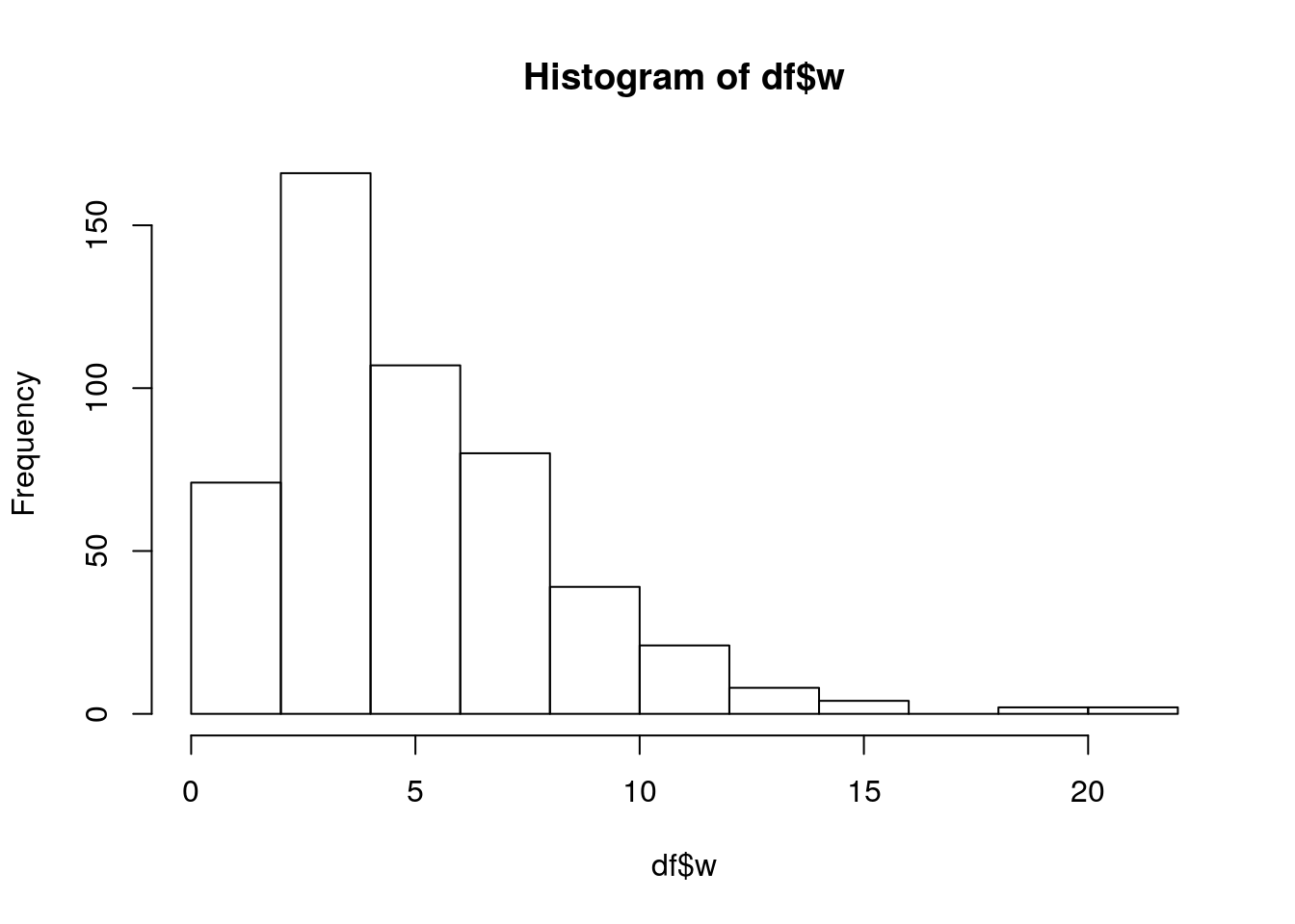
5.4 Write a new function in R
The Do not repeat yourself (DRY) principle suggests avoiding repetitions in the code, as copy-and-paste the same code to compute the same quantity(ies) for different data, as we did previously for the skewness index. The more repetition you have in your code, the more places you need to remember to update when things change, and the more likely you will include errors in your code.
Automate common tasks through functions is a powerful alternative to copy-and-paste. When input changes, with functions you only need to update the code in one place instead of many (this eliminates the chance of incidental mistakes).
To define a new function we use the following structure: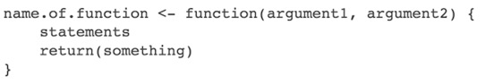
Figure 5.1: How to define a new function with 2 inputs in R
For the computation of the skewness index we define a new function named myskew which takes in input the vector named x (this is a name chosen by us, you could use choose a different one). This is the function definition:
myskew = function(x){
  mean((x - mean(x))^3) / sd(x)^3
}
The function automatically returns the output of the last computation.
After running the code, you will see a new object of type function in the top right panel. It is now possible to apply the function to a single column of df:
myskew(x = df$x)## [1] -0.1391724#omit the argument name
myskew(df$x)## [1] -0.1391724You can even use myskew inside apply and compute the skewness jointly for all the columns:
apply(df, 2, myskew)## x y z w
## -0.13917239 0.00426134 -0.20619759 1.36738140Note that by default the function returns the value of the last evaluated expression (the value of the skewness index in this case). Let’s assume that we want to define a new function which returns the values of the skewness and kurtosis indexes. In this case the output is a vector of two values (s and k representing the skewness and kurtosis index, respectively) and it can be returned by using the return function:
myskewkur = function(x){
  s = mean((x - mean(x))^3) / sd(x)^3
  k = mean((x - mean(x))^4) / sd(x)^4
  return(c(s,k))
}
Let’s now apply the function myskewkur to a single column of df and to all its column by using apply:
myskewkur(df$x)## [1] -0.1391724 2.7668950apply(df, 2, myskewkur)## x y z w
## [1,] -0.1391724 0.00426134 -0.2061976 1.367381
## [2,] 2.7668950 1.82261893 6.0524876 5.895259We can observe that the output is not labeled. It is possible to obtain a labeled output by changing the returned vector and including labels:
myskewkur = function(x){
  s = mean((x - mean(x))^3) / sd(x)^3
  k = mean((x - mean(x))^4) / sd(x)^4
  return(c("skewness" = s,"kurtosis" = k))
}
The output now is completely specified:
myskewkur(df$x)## skewness kurtosis
## -0.1391724 2.7668950apply(df, 2, myskewkur)## x y z w
## skewness -0.1391724 0.00426134 -0.2061976 1.367381
## kurtosis 2.7668950 1.82261893 6.0524876 5.895259When the output to return is more complex you will need to use a list. Let’s consider for example that, besides computing the skewness and the kurtosis, we want our function to simulate (and return) \(n\) values simulated from the Normal distribution with mean/sd equal to the empirical mean/sd of the considered vector. The term \(n\) represents the second argument of the function and its value will be specified later by the user when the function is applied.
myskewkursim = function(x, n){
# Compute the skewness and the kurtosis
s = mean((x - mean(x))^3)/sd(x)^3
k = mean((x - mean(x))^4)/sd(x)^4
# Simulate the values
d = data.frame(x = rnorm(n,
mean(x),
sd(x)))
# Return your output using a named list
return(list(summarystats = c(skewness = s, kurtosis = k),
simulationdf = d))
}In the above defined function the output will be a list with two components:
- a vector composed by two values (skewness and kurtosis)
- a data frame named simulationdf with a single column named x
Let’s apply the function to a column of df:
myoutput = myskewkursim(df$x, n=10)
myoutput## $summarystats
##   skewness   kurtosis
## -0.1391724  2.7668950
##
## $simulationdf
## x
## 1 -1.0617293
## 2 0.3912956
## 3 0.6661875
## 4 -0.3752550
## 5 0.4538922
## 6 -0.1871766
## 7 1.0029827
## 8 -0.8206790
## 9 0.8813049
## 10 0.3256912The object myoutput is of type list and contains the following elements:
length(myoutput)## [1] 2names(myoutput)## [1] "summarystats" "simulationdf"It is now possible to perform subsequent analysis on this output. We could, for example, plot the simulated values contained in the column x of simulationdf:
myoutput$simulationdf$x## [1] -1.0617293 0.3912956 0.6661875 -0.3752550 0.4538922 -0.1871766
## [7] 1.0029827 -0.8206790 0.8813049 0.3256912hist(myoutput$simulationdf$x)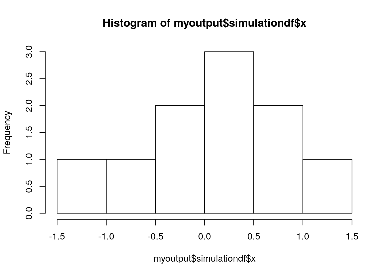
The function myskewkursim can also be embedded inside apply in order to apply it jointly to all the columns of df:
myoutput2 = apply(df, 2, myskewkursim, n=10)In this case the output is more complex and given by a list of lists:
# outer list
class(myoutput2)
## [1] "list"length(myoutput2)## [1] 4# the first element of the outer list
class(myoutput2[[1]])## [1] "list"length(myoutput2[[1]])## [1] 25.5 Conditional statements
Let’s say that we want now to expand the myskew function and include the possibility to plot the distribution of x. The user will have the possibility to choose the type of plot between boxplot, histogram, and kernel density plot. Thus, we need to include a new argument in the function definition regarding the plot type; moreover, in the function of the body we will have to include a conditional statement which performs a different action (i.e. produce a plot) according to the available alternatives (boxplot, histogram and otherwise). The general definition for a conditional statement is the following:
It is also possible to test more conditions:
if (condition1){
  expr1
  #code executed when condition1 is TRUE
} else if (condition2){
  expr2
  #code executed when condition2 is TRUE
} else if (condition3) {
  expr3
  #code executed when condition3 is TRUE
} else {
  expr 4
  #code executed otherwise
}
For the specific case we will have
myskewplot = function(x, plottype){
  s = mean((x - mean(x))^3)/sd(x)^3

  if(plottype == "boxplot"){
    boxplot(x)
  } else if(plottype == "histogram"){
    hist(x)
  } else { #otherwise
    plot(density(x))
  }
  return(s)
}
The function can be used as follows:
myskewplot(x=df$x,
           plottype = "boxplot")
## [1] -0.1391724myskewplot(x=df$x,
plottype = "somethingelse")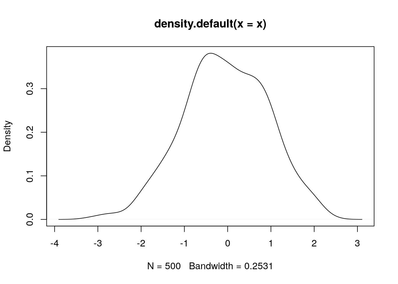
## [1] -0.1391724Note that if the user doesn’t specify the plottype (e.g. myskewplot(df$x)) the function will return an error. It could be useful in this case to set a default option for the plottype argument so that the function will works even if no choice is expressed for the type of plot:
myskewplot = function(x, plottype = "boxplot"){
  mean((x - mean(x))^3)/sd(x)^3

  if(plottype == "boxplot"){
    boxplot(x)
  } else if(plottype == "histogram"){
    hist(x)
  } else {
    plot(density(x))
  }
}
myskewplot(df$x)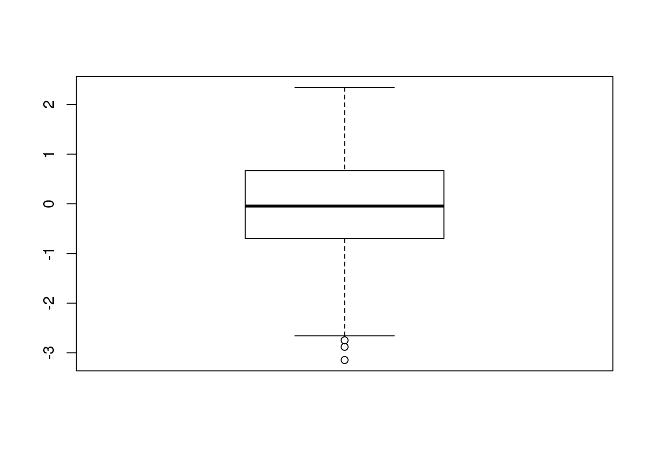
A simplified version of a conditional statement if given by the ifelse function (see also ?ifelse). This function performs a test and then perform two different actions according to the test output. In case be useful for example to
transform the variables df$z into a new variable which is equal to 0 if z>0 and equal to 1 otherwise. The new variable will be saved in a new column named z2:
df$z2 = ifelse(df$z > 0, 0, 1)
head(df)
## x y z w z2
## 1 -0.2409516 6.4480150 -1.1082764 2.464180 1
## 2 -0.5004062 9.9065245 -2.3763105 6.582193 1
## 3 -0.3952414 3.4989756 -1.4033463 5.045619 1
## 4 -0.7952692 0.9429413 0.7804105 4.606289 0
## 5 0.5399611 5.1325526 0.8343994 4.209044 0
## 6 1.4889313 5.1903847 2.1541173 2.229942 0table(df$z2) #frequency distribution##
## 0 1
## 257 243Instead of using the 0 and 1 categories, another possibility is to use two categories like positive and negative:
df$z3 = ifelse(df$z > 0, "positive", "negative")
head(df)
## x y z w z2 z3
## 1 -0.2409516 6.4480150 -1.1082764 2.464180 1 negative
## 2 -0.5004062 9.9065245 -2.3763105 6.582193 1 negative
## 3 -0.3952414 3.4989756 -1.4033463 5.045619 1 negative
## 4 -0.7952692 0.9429413 0.7804105 4.606289 0 positive
## 5 0.5399611 5.1325526 0.8343994 4.209044 0 positive
## 6 1.4889313 5.1903847 2.1541173 2.229942 0 positivestr(df)## 'data.frame': 500 obs. of 6 variables:
## $ x : num -0.241 -0.5 -0.395 -0.795 0.54 ...
## $ y : num 6.448 9.907 3.499 0.943 5.133 ...
## $ z : num -1.108 -2.376 -1.403 0.78 0.834 ...
## $ w : num 2.46 6.58 5.05 4.61 4.21 ...
## $ z2: num 1 1 1 0 0 0 1 0 1 0 ...
## $ z3: chr "negative" "negative" "negative" "positive" ...table(df$z3)##
## negative positive
## 243 2575.6 For loop
When you want perform some computation repetitively you can use a for loop generally coded as follows:
for(i in sequence){
     expression 1
     expression 2
}
where i is the index variable and sequence is the vector of (integer) values taken by the index (usually represented by a regular sequence). All the expressions enclosed in braces are repeatedly evaluated as i ranges through the values in the sequence vector.
Let’s consider for example the case of \(m=5\) different Normal random variable characterized by different mean values (equal to \(1,2,\ldots,m\)) but the same variance (equal to 1).
For each random variable (\(1,2,\ldots,m\)) we want to 1. simulate \(n=100\) values from the random variable 2. save the simulated values in a list 3. compute the coefficient of variation (sd/mean) and save the value in a vector
We thus have to repeat the same three operations for \(m\) random variables (and we don’t want to use code copy-and-paste!).
We start by defining the needed objects:
m = 5 #number of Normal RV
n = 100 #number of values to simulate

# Vector of the mean values for the m RVs
mean_vec = 1:m #regular sequence of integers from 1 to m
mean_vec
## [1] 1 2 3 4 5We also prepare the empty objects (a list and a vector) where we will save the output iteration by iteration sequentially:
# empty list
sim_list = list()
# empty vector
cv_vec = c()
We are now ready to write the for loop:
for(i in 1:m){

  sim = rnorm(n, mean=mean_vec[i], sd=1)
  #the mean changes at each iteration!

  # save the vector in the i-th position of the list  sim_list
  sim_list[[i]]  = sim

  # save the cv value in the i-th position of the vector cv_vec
  cv_vec[i] = sd(sim)/mean(sim)
}
After running the for loop the list and the vector will contain \(m\) objects, respectively:
cv_vec## [1] 0.8738922 0.4759851 0.3435681 0.2129892 0.2027989sim_list## [[1]]
## [1] 0.112467586 -1.685752519 0.960809736 1.682911839 1.601306095
## [6] 1.112192926 0.851118000 1.026733701 1.883761159 1.237355332
## [11] 0.463471580 2.118097759 1.878052076 1.981477107 -0.296101559
## [16] -0.750467172 2.349552590 1.016278948 0.934392377 0.578853377
## [21] 1.894230655 -0.198286925 2.219417990 3.224032676 2.056962432
## [26] 0.340782191 1.384027000 1.604703764 1.076206949 -0.408176052
## [31] -1.028346671 1.318337765 1.978728501 0.579734678 -0.303021467
## [36] 1.361241386 0.614914561 1.656504557 1.172073543 3.541517153
## [41] 1.970598951 0.576590356 1.241501425 0.659240118 1.377941460
## [46] 3.550126249 0.654095632 0.891477845 1.047966959 3.959816626
## [51] -0.909914673 1.340954881 2.452644752 1.816460790 0.817881212
## [56] 0.407097712 0.883509579 -0.609234964 0.298196177 1.248725541
## [61] 0.735020339 -0.368584142 1.197602398 1.041762473 1.652987655
## [66] 2.012708510 0.904167789 0.744771063 1.767463187 1.608377807
## [71] 4.023025918 0.309706801 -0.001202014 0.227420103 2.345672468
## [76] 3.082064967 0.782786122 1.773778692 0.919541113 1.725650363
## [81] 1.246961880 1.121220166 0.948646155 1.818587240 2.043123234
## [86] 1.065713960 0.498318332 1.367291037 1.506689705 1.931294702
## [91] 1.891230288 1.471280099 0.267500899 2.283787879 0.706828585
## [96] 0.139239142 1.417238417 1.296622694 1.309647817 -0.511906303
##
## [[2]]
## [1] 2.88997405 0.38811704 1.30162713 1.21994938 1.69723321 1.49131331
## [7] 1.65374522 1.54452546 2.96934293 0.94208332 1.65359424 3.21142253
## [13] 2.47090592 4.07018305 2.01918177 1.48045717 2.51968148 1.71236906
## [19] 0.97360683 0.34200037 0.60272943 3.54337675 2.65053002 3.32702553
## [25] 2.14661322 2.36020777 0.98707837 1.89205325 0.78736463 1.63589767
## [31] 2.02651182 -0.56359402 0.24489206 2.44691979 0.62979878 1.77861542
## [37] 2.85963818 1.88373182 2.35326143 2.26600504 2.59576986 0.03873814
## [43] 2.29321281 -0.32185134 2.00197782 2.05670977 2.50948711 2.55151004
## [49] 2.03116218 2.46536101 1.29459930 1.97374930 0.64436552 2.05094205
## [55] 3.29766719 2.94347378 2.42653498 1.53631939 1.31042750 3.25126786
## [61] 3.28654781 1.65857604 1.20906896 3.14610704 3.17272199 1.88169917
## [67] 0.83955532 1.60615682 1.31227457 2.14964222 2.01568176 0.88565506
## [73] 2.49085712 2.34989472 2.25232682 0.97785076 2.67884095 1.61156301
## [79] 1.52972581 2.28126199 1.48703326 3.00762353 1.37810118 2.38439725
## [85] 2.39577030 2.88442037 2.97835910 1.25634088 1.13973782 1.81550909
## [91] 1.16947402 1.14086043 2.10888493 2.72896325 1.03291068 2.54359789
## [97] 0.25404713 1.18443062 2.92372854 2.32079355
##
## [[3]]
## [1] 1.8945120 0.6563211 4.2225950 3.7990285 1.7216680 2.2750597 2.7281603
## [8] 3.1809734 2.2267318 4.1776417 3.8132880 2.6447648 4.0645681 2.4166886
## [15] 3.3288051 2.9224226 3.4386177 2.2337279 5.3169508 4.2597029 2.7449321
## [22] 1.4816254 3.3046810 3.0832828 2.6581017 2.8690683 3.7350686 2.2783440
## [29] 4.7531613 2.3191388 1.1831414 3.2373913 5.2995614 4.1508033 1.9498252
## [36] 1.2261558 2.9900579 3.3641532 2.3022830 4.1844134 1.3721699 2.9965199
## [43] 2.1243371 3.1905904 3.0756414 3.3209532 1.7567988 4.0299000 2.2970213
## [50] 3.0525502 1.4480348 1.9668753 2.9437881 3.5512039 2.5336977 3.4169009
## [57] 2.7979230 2.9176155 1.9698062 2.6988948 1.9310383 2.6964530 1.6945254
## [64] 2.3334788 4.1814151 2.6567623 4.5888436 2.9473920 1.8170631 2.0751781
## [71] 3.4634494 3.2985974 2.3856687 1.6365666 4.2190864 2.2525656 2.8777096
## [78] 2.7839944 3.0210228 2.9531584 1.2347157 3.6005078 2.5620664 1.5899887
## [85] 2.3203393 2.6857658 0.7780985 2.3372300 2.4413044 3.1534862 1.6081316
## [92] 3.5842612 2.5587315 4.2155118 1.8399311 3.7374900 4.5872929 3.9702635
## [99] 4.8250140 3.5746206
##
## [[4]]
## [1] 5.287979 4.042479 3.365411 3.249000 3.197662 3.067225 3.858432 4.583878
## [9] 5.018925 4.553308 4.000206 3.383911 2.628825 4.052402 3.505019 4.528775
## [17] 3.979862 3.302058 3.348394 3.574504 4.249096 2.830893 3.092711 3.959691
## [25] 4.006791 4.746315 3.600120 6.067058 3.797528 4.174671 3.638800 3.283086
## [33] 3.056250 4.889915 3.824587 4.950779 3.823940 2.166758 2.830818 3.836162
## [41] 4.062235 2.953773 5.279956 3.259102 4.195291 4.447665 2.535701 4.404182
## [49] 3.773048 5.342606 4.122551 4.641074 3.692265 4.894723 4.210336 2.178621
## [57] 3.311538 2.883355 4.567586 5.557555 3.164870 3.406800 2.667704 3.248737
## [65] 4.793209 4.237753 2.896356 3.777737 5.483793 3.564498 3.993683 3.580689
## [73] 4.493259 5.129077 3.546769 3.385959 2.729214 4.019723 3.346041 4.782494
## [81] 2.950127 4.240778 5.411590 2.816554 3.694839 3.332051 4.808171 3.383445
## [89] 3.511144 3.476817 4.434708 5.511146 3.842480 5.156386 3.261030 4.024398
## [97] 3.329417 2.514899 3.639798 3.280532
##
## [[5]]
## [1] 4.960572 5.484061 5.586146 4.254962 4.635550 4.167298 5.003161 5.567554
## [9] 5.132502 3.934465 4.649018 4.659036 6.452036 4.933314 6.368143 4.877511
## [17] 5.616786 6.849743 5.016845 6.490217 5.341052 3.521392 5.316325 4.500873
## [25] 3.916107 4.080635 5.625622 5.320912 7.191865 5.514768 5.926317 5.976223
## [33] 4.614937 3.454322 6.042708 6.941604 1.459588 4.876672 3.972809 5.201990
## [41] 6.008757 4.954881 5.095024 4.423756 4.052520 4.855524 3.546431 5.370870
## [49] 3.980605 4.705431 4.626666 4.952334 6.702002 4.287973 4.471741 3.882515
## [57] 4.702322 4.013439 4.925250 5.573306 2.839681 5.938378 4.238518 5.979064
## [65] 5.643195 5.527218 5.038894 5.729660 4.883399 3.625731 5.184318 4.339343
## [73] 6.445496 4.889987 4.000855 3.296403 5.086217 6.310122 4.697260 5.635539
## [81] 5.104809 6.731753 3.217572 4.745606 5.234381 3.885542 4.296661 5.608260
## [89] 3.875526 4.122327 3.738682 6.714334 5.005814 4.871702 4.515647 4.358515
## [97] 4.455844 3.754081 6.880849 4.186891Note that in this case the sim_list list doesn’t have names that can be however set later. First of all note that at the moment there are no names for the list
names(sim_list)## NULLLet’s say that we want to set the following names for the list: n1, n2, … n5 (so a common letter attached to a sequence of integers). For this we need to use the function paste:
paste("n", 1:m, sep="")## [1] "n1" "n2" "n3" "n4" "n5"Finally we set the list names:
names(sim_list) = paste("n", 1:m, sep="")
names(sim_list)
## [1] "n1" "n2" "n3" "n4" "n5"We could then plot the distribution given in the first element of the list:
hist(sim_list[[1]])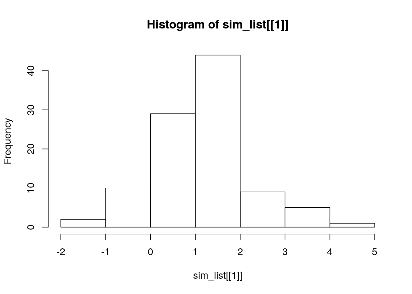
5.7 Exercises Lecture 3
5.7.1 Exercise 1
- Consider the following list:
a = list (x=5, y=10, z=15, w=rnorm(10))
a
## $x
## [1] 5
##
## $y
## [1] 10
##
## $z
## [1] 15
##
## $w
## [1] -1.09832672 1.31653973 -0.91559581 -0.37087810 -0.85180641 -0.05625113
## [7] -1.86185160 0.50613153 -1.63551386 0.05409524- Compute the sum of all the elements in
a. - Extract the second element of
w. - Compute how many elements of
ware positive. - Comment the following code:
q = sample(letters[1:5], 20, replace=T)
qf = factor(q)
class(qf)
## [1] "factor"table(qf)## qf
## a b c d e
## 6 4 3 3 4levels(qf)## [1] "a" "b" "c" "d" "e"a$qf = qf
a## $x
## [1] 5
##
## $y
## [1] 10
##
## $z
## [1] 15
##
## $w
## [1] -1.09832672 1.31653973 -0.91559581 -0.37087810 -0.85180641 -0.05625113
## [7] -1.86185160 0.50613153 -1.63551386 0.05409524
##
## $qf
## [1] d c a e a e c a b d d b a a a b c b e e
## Levels: a b c d e- Consider the following list:
b = list(x=1:10, b="Good morning", c="Hi")Add 1 to each element of the first object in b.
5.7.2 Exercise 2
Define a function named
mypowerto print a number raise to another. The two numbers are the arguments of the function and the exponent number is set by default equal to one.Compute using
mypowerthe following quantities: \(2^3\), \((\exp(4))^{\sqrt{5}}\), \(\log(45)\).Is it possibile to provide a vector of exponents as input to the
mypowerfunction (while the base doesn’t change)? If yes, provide and example.
5.7.3 Exercise 3
- Define a function named
myfwhich takes a single argument \(x\) and returns the value of the function \(f(x)\) which is defined as follows:
- \(f(x)=x^2+2x+3\) if \(x<0\);
- \(f(x)=x+3\) if \(0\leq x <2\);
- \(f(x)=x^2+4x-7\) if \(x\geq 2\).
- Evaluate the function in the following values of \(x\): -4.5, 5.90, 122.
5.7.4 Exercise 4
Define a function which computes, given a sample of \(n\) data, the confidence interval with confidence level \(1-\alpha\) for the unknown mean of the population where the sample is drawn from. For \(1-\alpha\) use 0.95 as default value. Remember that the formula for the confidence interval is given by the following formula: \[\left(\bar x -z_{\alpha/2}\frac{s}{\sqrt n};\bar x +z_{\alpha/2}\frac{s}{\sqrt n}\right)\] where \(\bar x\) is the sample mean (
mean), \(s\) the sample standard deviation (sd), \(n\) the sample size and \(z_{\alpha/2}\) the quantile of the standard Normal distribution which has an area equal to \(1-\alpha/2\) on the left side (use the functionqnormto compute it; see?qnorm).Apply the function to a vector of 600 numbers simulated from a Normal distribution with mean equal to 5 and variance equal to 1. For simulating the data use 444 as seed value.
5.7.5 Exercise 5
Create a function
wt_meanwhich compute the weighted mean given by this formula \[\bar x = \frac{\sum_{i=1}^n x_iw_i}{\sum_{i=1}^n w_i}\] where \(x_i\) is the generic value of the variable and \(w_i\) the corresponding weigth (\(i=1,\ldots,n\)). This function will have two vectors as input (one for the data and one for the weights) and you have to check they they have the same length, otherwise the function will have to stop and exit with an error message (for this you can usestop, see?stop).Test the function with the following data (exam grades) and weights (exam credits):
Test the function with the following data (exam grades) and weights (exam credits):
5.7.6 Exercise 6
- Implement a
ratiofunction which takes a single number as input. If the number is divisible by three, it returns “Divisible by 3” (you can use theprintfunction). If it’s divisible by five it returns “Divisible by 5”. If it’s divisible by three and five, it returns “Divisible by 3 and 5”. Otherwise, it returns the number. Use the modulo operator%%to check divisibility. The expressionx %% yreturns 0 ifydividesx. See the following example:
4 %% 2 #4 is divisible by 2## [1] 05 %% 2 #5 is not divisible by 2## [1] 1Run the
ratiofunction with the following numbers: 33, 50, 150, 46570, 9877.Define the object
y=round(runif(1,0,1000),0). Then run (many times) theratiofunction with the valuey.
5.7.7 Exercise 7
- How could you use
cutfunction to simplify this set of nested if-else statements? See?cut. Suggestion: use-InfandInffor the lowest and highest value.
temp = 22.5

if (temp <= 0) {
  "freezing"
  } else if (temp <= 10) {
  "cold"
  } else if (temp <= 20) {
  "cool"
  } else if (temp <= 30) {
  "warm"
  } else {
  "hot"
}
## [1] "warm"- Run the code with
cutwith a vector of temperature, e.g.runif(15, -30,60). Provide the absolute frequencies for the qualitative variable with 5 categories.
5.7.8 Exercise 8
Consider the following vector of sample sizes (see the help of the function seq):
samplesize_vec = seq(1, 5000, by=100)
samplesize_vec
## [1] 1 101 201 301 401 501 601 701 801 901 1001 1101 1201 1301 1401
## [16] 1501 1601 1701 1801 1901 2001 2101 2201 2301 2401 2501 2601 2701 2801 2901
## [31] 3001 3101 3201 3301 3401 3501 3601 3701 3801 3901 4001 4101 4201 4301 4401
## [46] 4501 4601 4701 4801 4901- For each sample size in the
samplesize_vec:
- simulate some values from the Normal distribution with mean equal to 2 and variance equal to 1 (the number of values to simulate is given by
samplesize_vecand change iteration by iteration) - compute the empirical mean and variance of the simulate values and save them in two different vectors.
- Plot (using the function
plot) the values in the two vectors. What do you observe?