6 Regression
This section covers regression analysis in the fixest package, written by Laurent Berge. While R has built-in regression functions (lm()), it also has many packages for regression analysis. Fixest is my favorite of these package for three main reasons.
- Fixest is flexible. With a single function (
feols), you can implement multivariate regression, fixed effects regressions, and even instrumental variables. It also has functionality for all of the common standard errors. You’ll rarely need any other regression package - Fixest is fast. This mainly matters when you’re amalyzing large datasets or implementing fixed effects regressions.19
- Fixest is pretty. The
etable()function is quick and easy way to make attractive, well-formatted output tables that summarize your results.
This section gives only a sparse introduction to fixest. For details, see the excellent documentation.
6.1 Fixest syntax
For our guiding examples, let’s use the bechdel dataset from fivethirtyeight. This dataset contains several variables about movie revenues and whether the movies pass the Bechdel test.20
library(fixest)
library(dplyr)
library(fivethirtyeight)

data('bechdel')

### Data processing
bechdel = bechdel %>%
  select(year, title, budget_2013, domgross_2013, clean_test) %>%
  mutate(clean_test = as.character(clean_test)) # get rid of factor labels

bechdel$random_number = runif(nrow(bechdel)) # random number

bechdel = na.omit(bechdel) #(drops all observations with NA values)

print(head(bechdel))
## # A tibble: 6 × 6
## year title budget_2013 domgross_2013 clean_test random_number
## <int> <chr> <int> <dbl> <chr> <dbl>
## 1 2013 21 & Over 13000000 25682380 notalk 0.0616
## 2 2012 Dredd 3D 45658735 13611086 ok 0.170
## 3 2013 12 Years a Slave 20000000 53107035 notalk 0.322
## 4 2013 2 Guns 61000000 75612460 notalk 0.327
## 5 2013 42 40000000 95020213 men 0.600
## 6 2013 47 Ronin 225000000 38362475 men 0.841Let’s implement a simple regression with domgross as the dependent variable and budget as the independent variable.
The main function in fixest is feols(). feols() accepts two key arguments and several options.
The first key argument is data, which is the dataset of interest. The second key argument is fml, which is the regression formula. When you write the fml argument, you use the syntax y ~ x. The dependent variable is to the left of the ~ symbol, the independent variables are to the right of the ~ symbol. All of the variables in your formula must be variables in the main dataset.
## OLS estimation, Dep. Var.: domgross_2013
## Observations: 1,776
## Standard-errors: IID
##                 Estimate   Std. Error  t value  Pr(>|t|)
## (Intercept) 3.615293e+07 3.781955e+06  9.55932 < 2.2e-16 ***
## budget_2013 1.056040e+00 4.822900e-02 21.89629 < 2.2e-16 ***
## ---
## Signif. codes:  0 '***' 0.001 '**' 0.01 '*' 0.05 '.' 0.1 ' ' 1
## RMSE: 111,733,102.8   Adj. R2: 0.212318
I use the summary() function to take an initial glance at the results. You can see the main regression statistics: coefficient estimates, standard errors, p-values, and an R-squred.
To implement a regression with multiple independent variables, simply add them (with +) to the right hand side of the ~ symbol in your fml argument. It is just like writing an equation!
results = feols(
  data = bechdel,
  fml = domgross_2013 ~ budget_2013 + random_number
)
summary(results)
## OLS estimation, Dep. Var.: domgross_2013
## Observations: 1,776
## Standard-errors: IID
## Estimate Std. Error t value Pr(>|t|)
## (Intercept) 3.505952e+07 5.987777e+06 5.855181 5.6653e-09 ***
## budget_2013 1.056380e+00 4.826400e-02 21.887515 < 2.2e-16 ***
## random_number 2.122016e+06 9.007658e+06 0.235579 8.1379e-01
## ---
## Signif. codes: 0 '***' 0.001 '**' 0.01 '*' 0.05 '.' 0.1 ' ' 1
## RMSE: 111,731,354.2 Adj. R2: 0.211898Often, you want to understand how a categorical variable is related to your dependent variable. In this case, you might want to understand how revenues correlate with the code for whether the film passed the bechdel test.
## [1] "notalk" "ok" "men" "nowomen" "dubious"In your econometrics class, you hopefully learned that you should create a set of dummy variables, one for each value of the categorical except for a left-out group, to conduct this analysis. Luckily for us, fixest automaticaly implements this sort of analysis if you include a character variable or a factor on the right hand side of a regression.
## OLS estimation, Dep. Var.: domgross_2013
## Observations: 1,776
## Standard-errors: IID
## Estimate Std. Error t value Pr(>|t|)
## (Intercept) 4.234370e+07 9.862962e+06 4.293203 1.8565e-05 ***
## budget_2013 1.039180e+00 4.887000e-02 21.264264 < 2.2e-16 ***
## clean_testmen -3.143348e+06 1.238325e+07 -0.253839 7.9965e-01
## clean_testnotalk 2.801307e+06 1.063853e+07 0.263317 7.9234e-01
## clean_testnowomen -8.766933e+06 1.338242e+07 -0.655108 5.1248e-01
## clean_testok -1.125089e+07 1.023483e+07 -1.099275 2.7180e-01
## ---
## Signif. codes: 0 '***' 0.001 '**' 0.01 '*' 0.05 '.' 0.1 ' ' 1
## RMSE: 111,565,230.5 Adj. R2: 0.212908clean_testmen is a dummy variable taking value 1 if clean_test == 'men' and 0 otherwise. The other clean_test variables are defined accordingly. For interpretation, always make sure you know the identity of the leave-out group. In this case, it is the clean_test == 'dubious' group.
To alter the leave-out group, we can make clean_test into a factor, and list the desired leave-out group first. In this case, we specify 'nowomen' as the leave-out group.
bechdel = bechdel %>%
mutate(clean_test =
factor(clean_test,
labels = c('nowomen', 'notalk', 'men', 'dubious', 'ok'))
)
results = feols(
  data = bechdel,
  fml = domgross_2013 ~ budget_2013 + clean_test
)
summary(results)
## OLS estimation, Dep. Var.: domgross_2013
## Observations: 1,776
## Standard-errors: IID
## Estimate Std. Error t value Pr(>|t|)
## (Intercept) 4.234370e+07 9.862962e+06 4.293203 1.8565e-05 ***
## budget_2013 1.039180e+00 4.887000e-02 21.264264 < 2.2e-16 ***
## clean_testnotalk -3.143348e+06 1.238325e+07 -0.253839 7.9965e-01
## clean_testmen 2.801307e+06 1.063853e+07 0.263317 7.9234e-01
## clean_testdubious -8.766933e+06 1.338242e+07 -0.655108 5.1248e-01
## clean_testok -1.125089e+07 1.023483e+07 -1.099275 2.7180e-01
## ---
## Signif. codes: 0 '***' 0.001 '**' 0.01 '*' 0.05 '.' 0.1 ' ' 1
## RMSE: 111,565,230.5 Adj. R2: 0.2129086.1.1 Accessing estimates
Sometimes, we want to do further computations with our model estimates. For example, to access coefficients from feols() result, use the following syntax: result$coefficients['variable_name']. Here is an example.
## budget_2013
##    1.039177
We created a variable key_estimate that contains a single coefficient estimate. You can modify it or use it however you like.
6.1.2 Fixed effects
For this section, I follow the example in Econometrics in R chapter 10. We use the dataset Fatalities from the AER package. That dataset contains traffic fatalities per year for each state, as well as several state-year level covariates. We will study the association between beer taxes and traffic fatalities.
library(fixest)
library(AER)
data(Fatalities)

Fatalities = Fatalities %>%
  mutate(
    fatal_rate_per_10K = fatal/pop*10000,
    year = as.numeric(year)
  ) %>%
  select(state, year, fatal_rate_per_10K, mormon, baptist,
         youngdrivers, miles, beertax, pop)

head(Fatalities)
## state year fatal_rate_per_10K mormon baptist youngdrivers miles beertax pop
## 1 al 1 2.12836 0.32829 30.3557 0.211572 7233.887 1.539379 3942002
## 2 al 2 2.34848 0.34341 30.3336 0.210768 7836.348 1.788991 3960008
## 3 al 3 2.33643 0.35924 30.3115 0.211484 8262.990 1.714286 3988992
## 4 al 4 2.19348 0.37579 30.2895 0.211140 8726.917 1.652542 4021008
## 5 al 5 2.66914 0.39311 30.2674 0.213400 8952.854 1.609907 4049994
## 6 al 6 2.71859 0.41123 30.2453 0.215527 9166.302 1.560000 4082999To include fixed effects, we only need to alter the fml argument to feols(). Any variables that we include after the | “vertical pipe” character are interpreted by R as fixed effects. See examples below.
out_year_as_variable = feols(
  data = Fatalities,
  fml = fatal_rate_per_10K ~ beertax + year
  )

out_fe = feols(
  data = Fatalities,
  fml = fatal_rate_per_10K ~ beertax | year
  )

print(out_year_as_variable)
## OLS estimation, Dep. Var.: fatal_rate_per_10K
## Observations: 336
## Standard-errors: IID
## Estimate Std. Error t value Pr(>|t|)
## (Intercept) 1.826302 0.074682 24.454353 < 2.2e-16 ***
## beertax 0.365631 0.062287 5.870088 1.0532e-08 ***
## year 0.006620 0.014860 0.445503 6.5625e-01
## ---
## Signif. codes: 0 '***' 0.001 '**' 0.01 '*' 0.05 '.' 0.1 ' ' 1
## RMSE: 0.541954 Adj. R2: 0.088461## OLS estimation, Dep. Var.: fatal_rate_per_10K
## Observations: 336
## Fixed-effects: year: 7
## Standard-errors: Clustered (year)
## Estimate Std. Error t value Pr(>|t|)
## beertax 0.366336 0.048247 7.59295 0.00027154 ***
## ---
## Signif. codes: 0 '***' 0.001 '**' 0.01 '*' 0.05 '.' 0.1 ' ' 1
## RMSE: 0.540533 Adj. R2: 0.079412
## Within R2: 0.094538Note the difference between the first table and the second. In the first regression, we are including year as a continuous numeric variable. R is trying to find the coefficients that best fit a model where the fatality rate depends linearly on both the beer tax and the year variable. In the second regression, we are including year as a fixed effect. R is making a set of dummy variables, one for each year except the leave-out group, and regressing the dependent variable on those. These are substantively different analyses and they result in different coefficient estimates on beertax.
As a rule of thumb, when you are working with panel data (i.e, when there are multpile units that appear in every year), you typically want to be implementing the second, fixed effects regression, rather than the first regression that only adjusts for a linear time trend.
You can also include multiple fixed effects. Add them to the formula on the right side of the |, just like you would for another independent variable.
out_twofe = feols(
  data = Fatalities,
  fml = fatal_rate_per_10K ~ beertax | year + state
  )
print(out_twofe)
## OLS estimation, Dep. Var.: fatal_rate_per_10K
## Observations: 336
## Fixed-effects: year: 7, state: 48
## Standard-errors: Clustered (year)
## Estimate Std. Error t value Pr(>|t|)
## beertax -0.63998 0.163126 -3.92322 0.0077731 **
## ---
## Signif. codes: 0 '***' 0.001 '**' 0.01 '*' 0.05 '.' 0.1 ' ' 1
## RMSE: 0.171819 Adj. R2: 0.891425
## Within R2: 0.036065Sometimes, you will want to use more exotic fixed effects, such as state times year effects.21 In these cases, visit the documentation, and control-F “interaction” for a comprehensive guide.
6.1.3 Alternative standard errors
For robust standard errors (as required throughout E3), include the option vcov = 'hetero'.
out_univariate_robust = feols(
  data = Fatalities,
  fml = fatal_rate_per_10K ~ beertax,
  vcov = 'hetero'
  )
To specify cluster-robust standard errors, use the cluster = option.
out_univariate_cluster = feols(
  data = Fatalities,
  fml = fatal_rate_per_10K ~ beertax,
  cluster = ~state
  )
For AR(1) standard errors (as required for the Gas Tax problem set in E3), you need to first tell R which dimension of your data is the “time” variable. You can do this with the panel() function, as below. Then, include the option vcov = NW(1) in your call to feols().22
6.2 Making tables with etable
The summary() outputs are quick to glance at, but for writeups it’s good to have tables that are easier for others to read. Enter etable(), which is the simplest flexible table formatting function I’ve found. It only works with fixest regressions.
result_list = list(out_univariate_robust, out_univariate_robust_weighted,
                   out_univariate_AR, out_fe)

setwd('./_book') # special line for image to render on website... will not matter for you.
etable(
  result_list,
  style.tex = style.tex('aer'),
  markdown = TRUE # special line for image to render on website
  )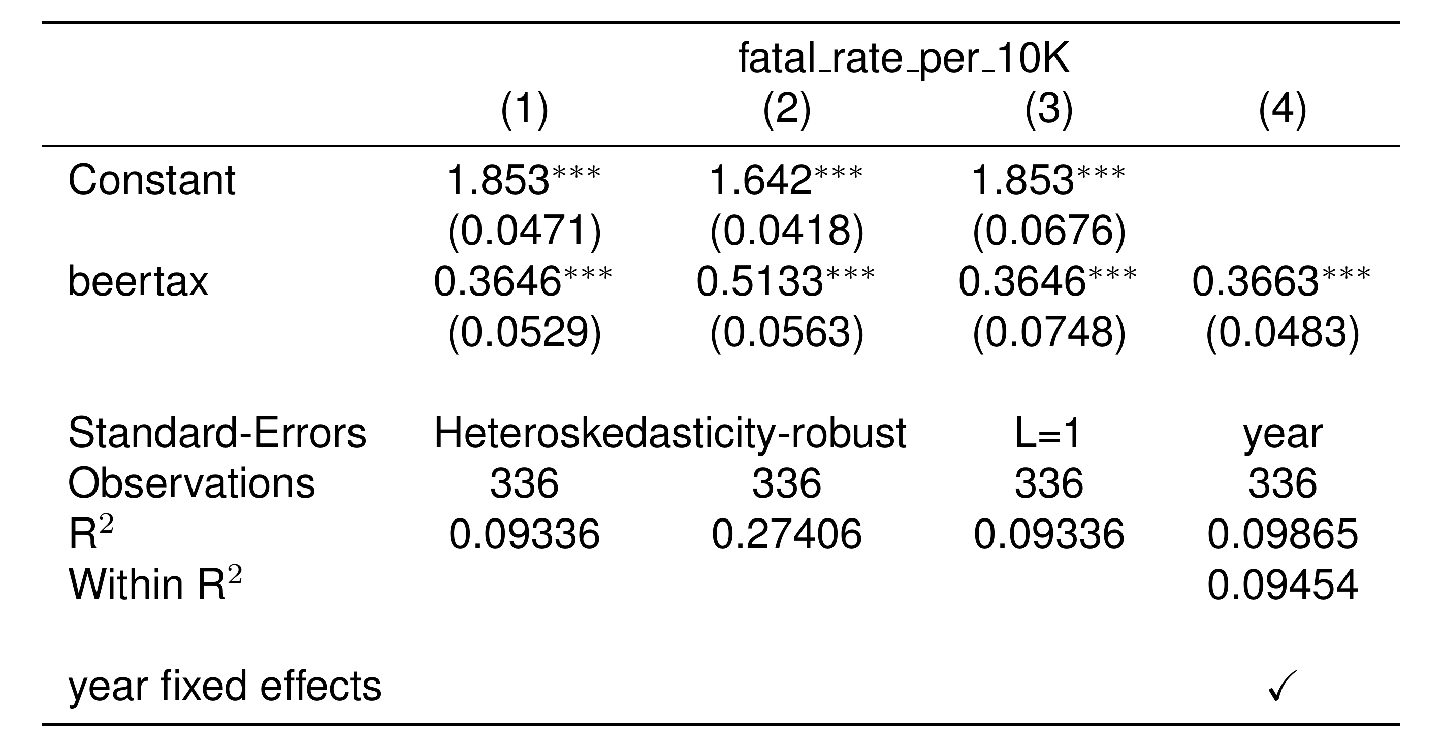
The first argument to etable is always a fixest result or a list of fixest results. This first argument is the only necessary input – all the other arguments specify table style.
6.2.1 Formatting
There are lots of ways to customize your tables – for example, you can see above that I’m asking the etable to follow the style guide of the American Economic Review. The fixest documentation contains a whole page about etable.
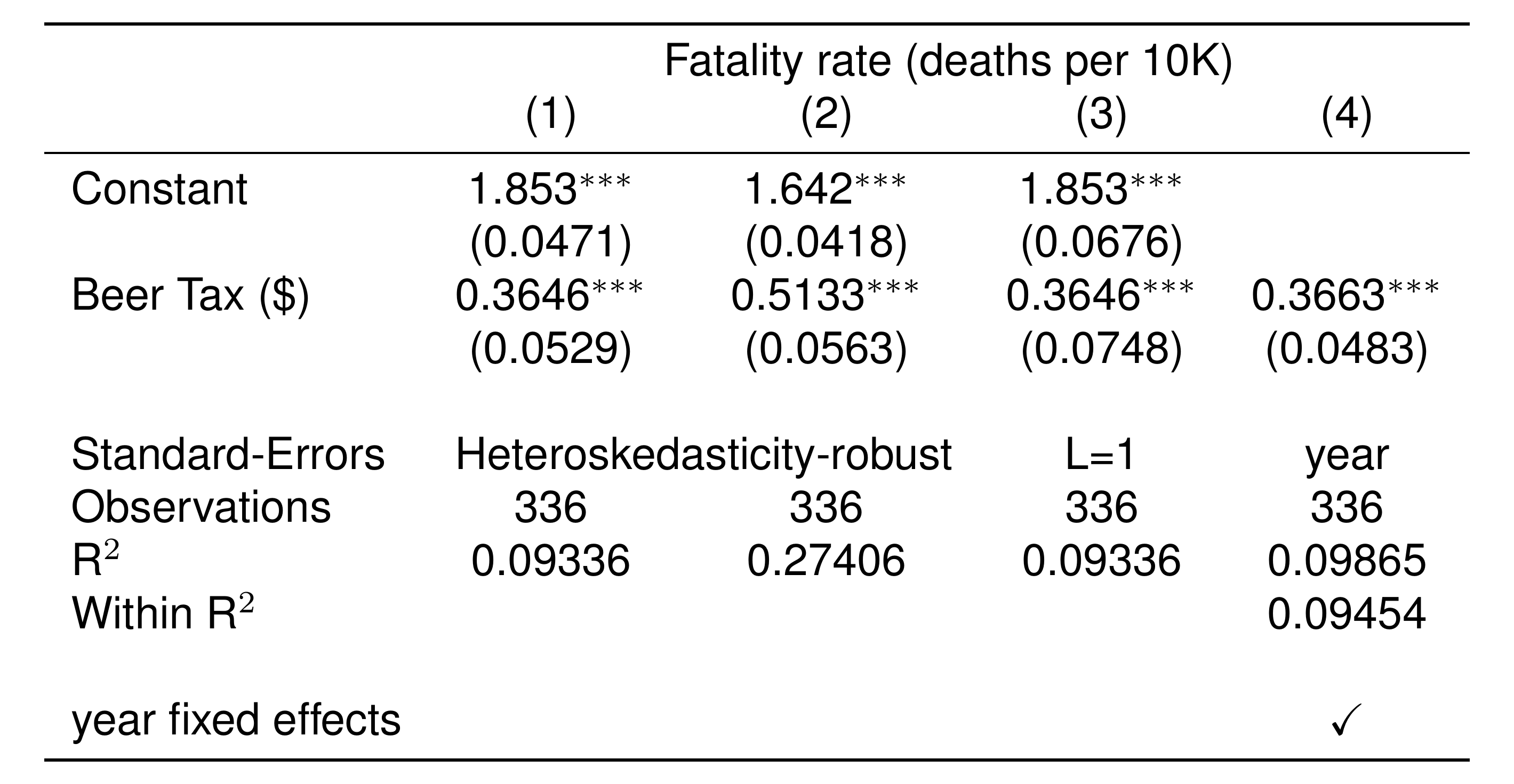
I will flag one important option: specifying your row names. You can see above that raw variable names appear in the table. That makes sense – R doesn’t know what else to call the variables! But when you present tables, you should make them easier to read. etable lets you change labels by setting a named character vector as a dictionary. You can make a dictionary like this.
dict_for_table = c(
  'beertax' = 'Beer Tax ($)',
  'fatal_rate_per_10K' = 'Fatality rate (deaths per 10K)'
)
The variable names are on the left side, and your labels are on the right side.
Then, when you run etable, you can pass your dictionary into the dict argument.
setwd('./_book') # special line for image to render on website... will not matter for you.
etable(
  result_list,
  style.tex = style.tex('aer'),
  dict = dict_for_table,
  markdown = TRUE # special line for image to render on website
  )
6.3 Instrumental variables
To estimate an IV regression, you again just have to change the fml input. fixest uses the following syntax: y ~ x_exog | FEs | x_endog ~ z, where…
yis the dependent variablex_exogare the exogenous variables (i.e, the variables you’re NOT instrumenting for)FEsare the fixed effectsx_endogare the endogenous variables (i.e, the variables you ARE instrumenting for)zare your instruments.
Essentially, everything is the same as before, except to do an IV you add another | and specify the first stage relationship to the right of that |. I give an example below, creating a random number to be the (fake) instrument.
setwd('./_book') # special line for image to render on website

Fatalities$random_number = runif(nrow(Fatalities))

res_IV = feols(
  data = Fatalities,
  fml = fatal_rate_per_10K ~ 1|state+year|beertax~ random_number,
  )

etable(
  res_IV,
  style.tex = style.tex('aer'),
  markdown = TRUE # special option for image to render on website
  )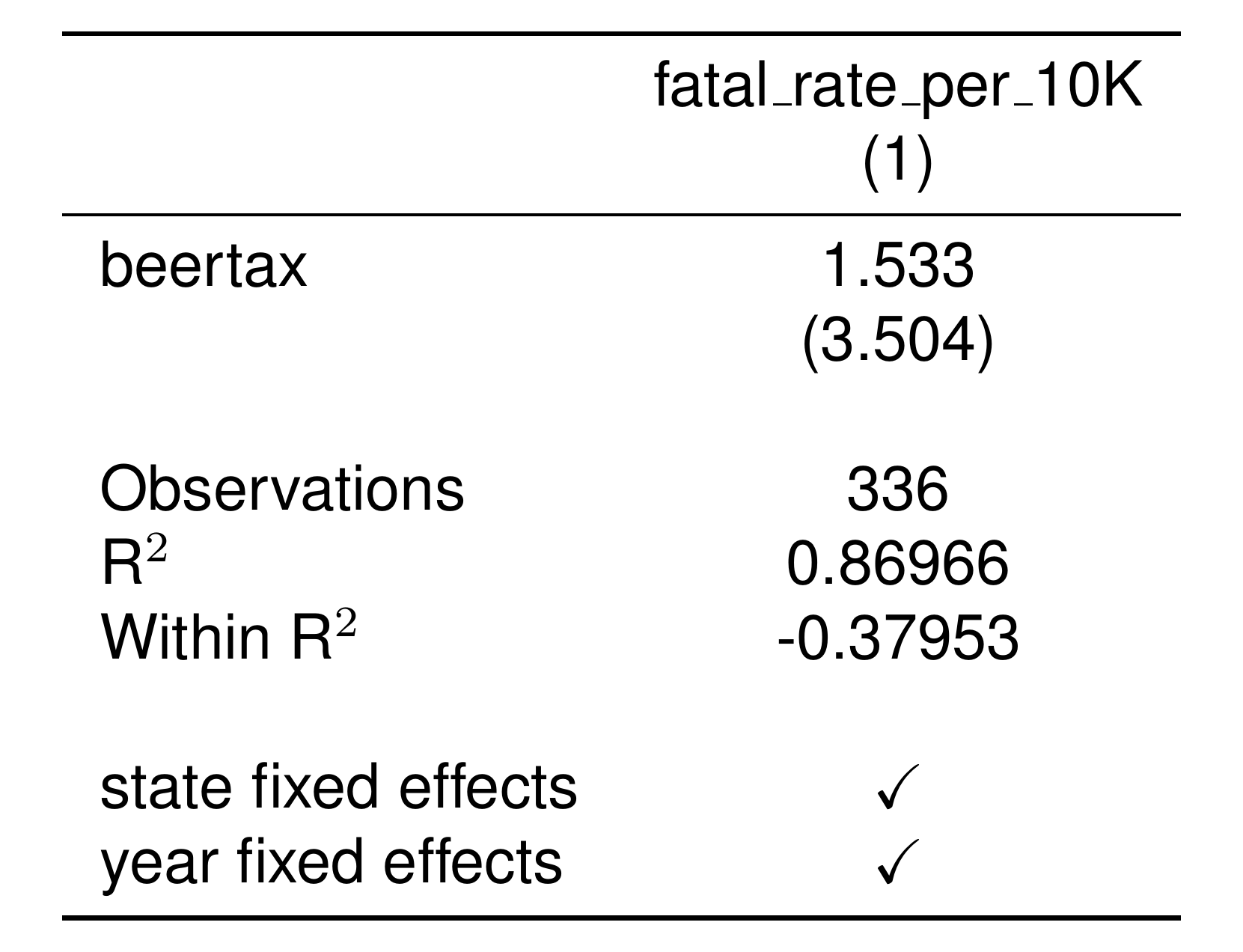
Note that because I did not have any exogenous RHS variables, I simply included the constant “1” as x_exog. This is a common trick – “1” denotes, “There are no variables in this part of the formula.” Similarly, if you want to do an IV analysis but you do not have any fixed effects, you can include a “1” after the first | divider.
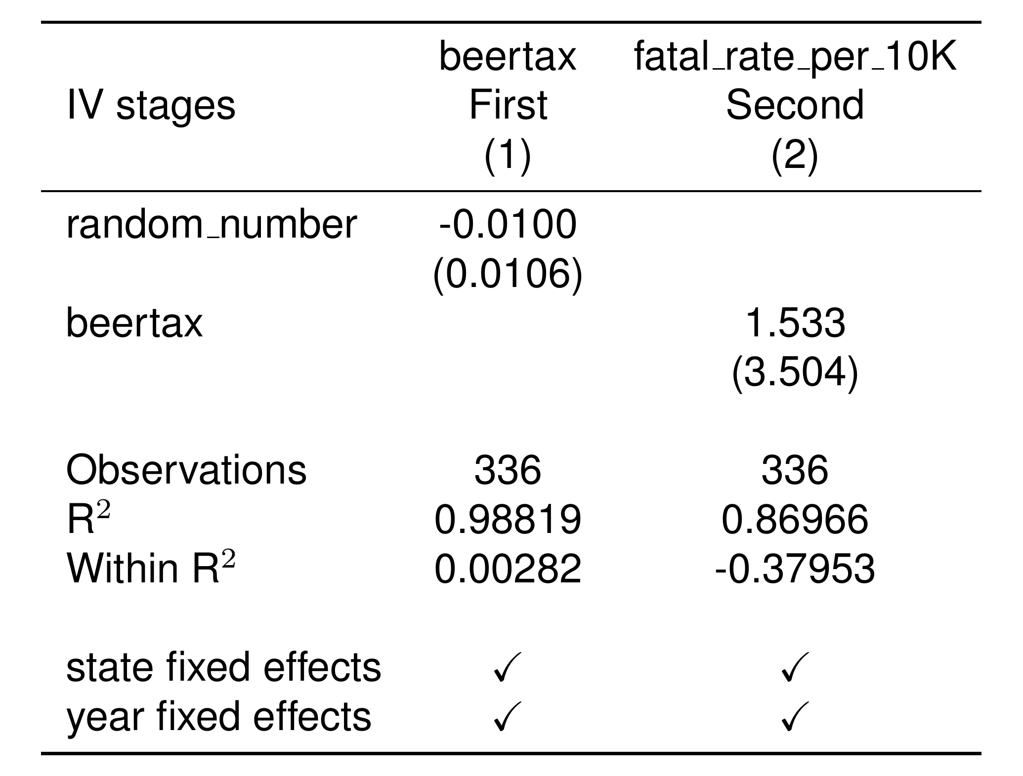
Here is a shortcut to have etable show both the first and second stage results simultaneously.
setwd('./_book') # special option for image to render on website

etable(
  res_IV, stage = 1:2,
  style.tex = style.tex('aer'),
  markdown = TRUE # special line for image to render on website
  )
There are several other shortcuts in fixest that you will discover as you become more familiar with it. You will rarely need another regression package.
6.4 Event studies
Event study plots are an extremely common visualization of results difference-in-difference style analyses. For details on event studies, see the relevant section of the Cunningham book, the discussion of dynamic difference in differences here, or this NBER working paper.
feols includes built-in tools that allow you to make attractive event study plots very quickly. For demonstration, feols includes a synthetic dataset called base_did with the following variables.
yan outcome variable (like “log house price” for an analysis of the treatment effects of Superfund cleanups on local house prices as in Greenstone and Gallagher (2008))idis a unit id (a census tract id in the example)periodis a time id (a year in the example)treatis an indicator for whether the unit got treated (an indicator for whether the tract got a cleaned in the example). In the example, the treatment takes place after period 5.
Many event study analyses include two plots. First, there’s a plot of the raw means over time for both groups.
library(ggplot2)
base_did = base_did %>%
  mutate(f.treat = factor(treat, labels = c('Treated', 'Control')))
ggplot(data = base_did,
       aes(x = period, y = y,  group = f.treat, color = f.treat)) +
  stat_summary_bin() +
  labs(x = 'Period', color = 'Group') +
  geom_vline(xintercept = 5.5, color = 'black', linetype = 'dashed')
## No summary function supplied, defaulting to `mean_se()`
## No summary function supplied, defaulting to `mean_se()`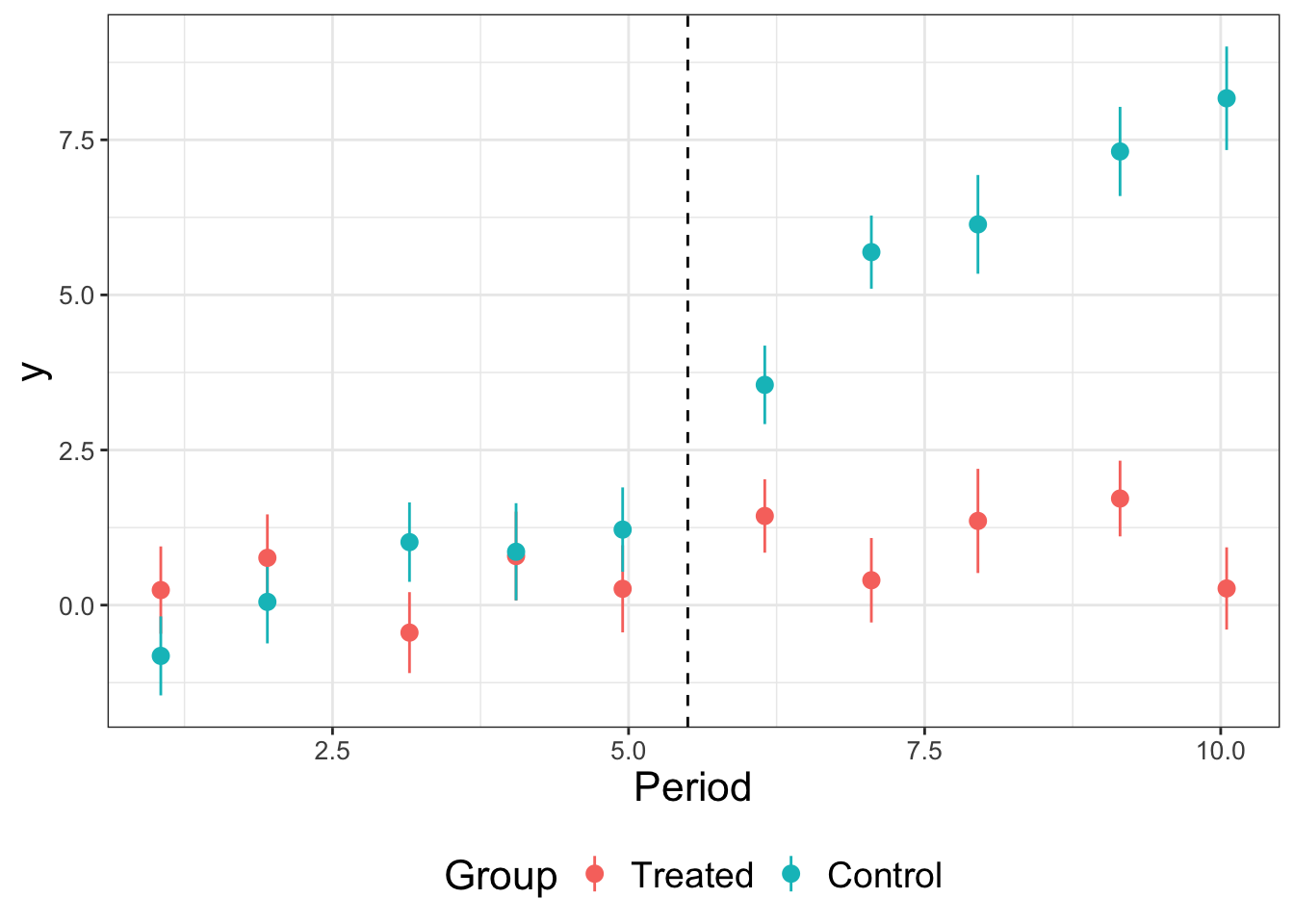
Next, the analyst plots the difference between the treated and control units over time, after controlling for unit fixed effects, period fixed effects, and potentially other within-unit variables that change over time. Typically these differences are comptuted with a regression:
This line says: “Regress y on unit fixed effects (id), time fixed effects (period), and then a set of period \(\times\) treatment indicators.” The function i(), which is part of the fixest package, creates these period \(\times\) treatment indicators. Specifically, it creates variables that are equal to 1 if and only if the observation is in a given period and the treat variable is 1. You must always specify one period to be the left-out or “reference” group. Traditionally, this is the period immediately before treatment, so here I specify it with ref = 5.
Here’s what the regression output looks like in a table.
setwd('./_book') # special line for image to render on website... will not matter for you.
etable(
  est_estud,
  style.tex = style.tex('aer'),
  dict = dict_for_table,
  markdown = TRUE # special line for image to render on website
  )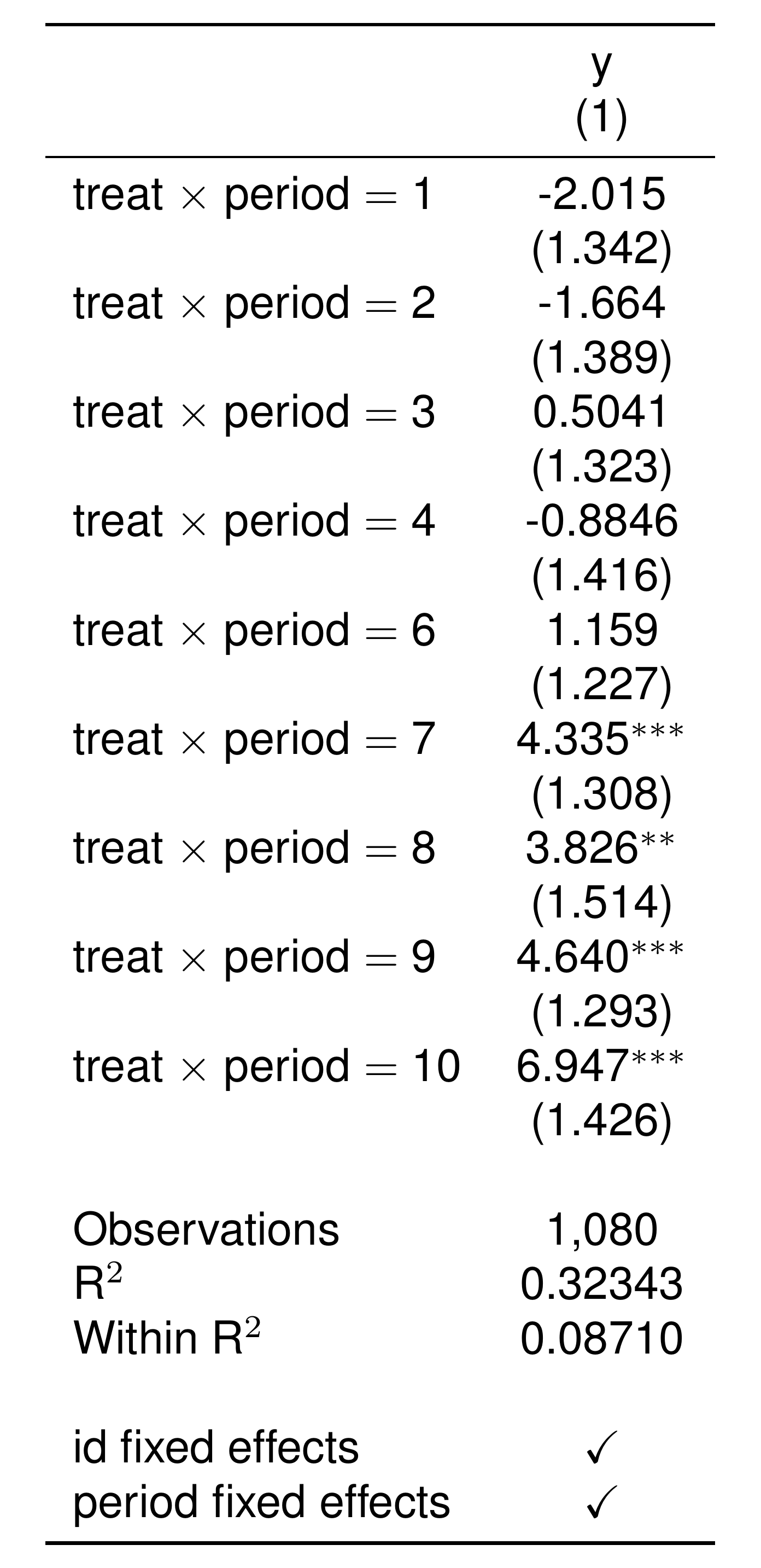
Note that there is no “treat \(\times\) period 5” variable, because we specified it as the left-out group.
To visualize the results, we use the wonderful ggiplot package.
require(ggiplot)
ggiplot(
  est_estud, main = 'Event Study Example') +
  labs(y = 'Effect (point estimate and 95% confidence interval', x = 'Period')+
  theme_bw()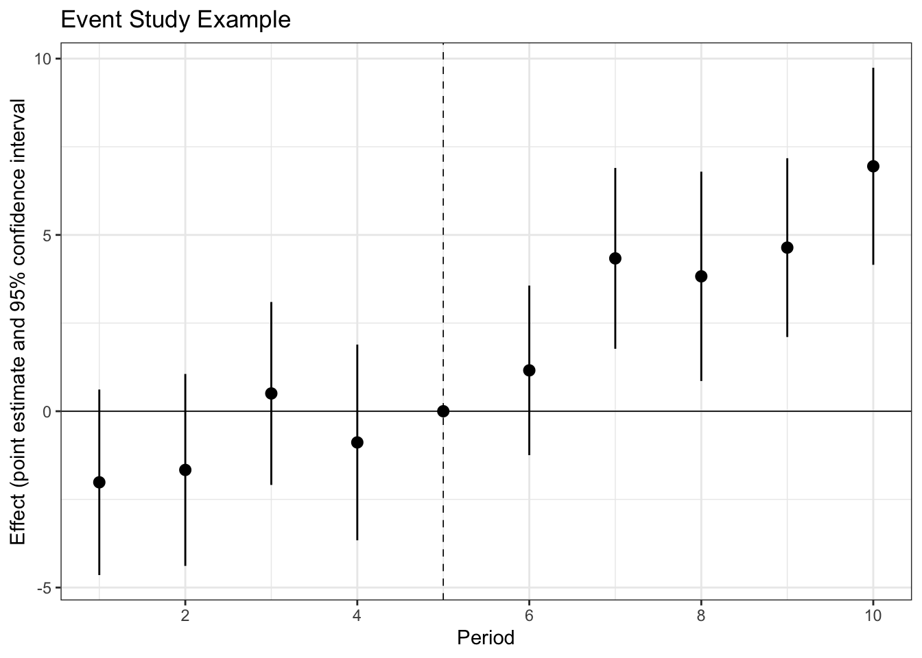
You can customize the look of your ggiplot just like it is a ggplot (by adding more layers). For more options, check out the vignettes on the website.
For E3 students, fixest will deliver time savings on the climate mortality problem set.↩︎
The relevant fivethirtyeight article explains more.↩︎
This comes up in the Climate Mortality PSet in E3, for example.↩︎
The NW stands for “Newey-West,” which is a way to compute AR standard errors.↩︎