5 Cleaning data
In this section, I give more details about data cleaning with the dplyr package. Throughout, I use two datasets from Opportunity Insights’s College Mobility Report Cards. An observation in the Opportunity Insights data is a U.S. college or university. Variables are characteristics of those universities. I use this example data to demonstrate strategies for several “data cleaning” tasks that are often required before analysis.
Here are descriptions of some key variables.
mr_kq5_pq1is the fraction of students whose parents are in the bottom quintile of the income distribution but who themselves end up in the top quintile of the income distribution. The authors of the paper use it as a measure of the extent to which a college encourages upward mobility.par_q1is a measure of the fraction of students at the college whose parents are in the bottom quintile of the income distribution.scorecard_netprice_2013is the average net cost of attendance for students recieving federal aid whose parents are at the bottom quintile of the income distribution.flagshipis an indicator for flagship state universities (e.g, Cal Berkeley)publicis an indicator for public institutions.hbcuis an indicator for a historically black college or university.
5.1 Loading data
I started by downloading the Opportunity Insights data from the internet, but now we need to load it into R.9
5.1.1 The working directory
R has a notion of a working directory, which determines how it tries to load files. Let’s look at an example. On my local computer, I stored the Opportunity Insights datasets in a folder called datasets/ – see the image below. That folder itself is contained in the folder bookdown-Rguide/, which is the folder where I have all the code I used to write this guide. And bookdown-Rguide/ is itself a subfolder of another folder… and so on. In the picture, I screenshotted the full list of folders, all the way back to the highest-level folder. This nested folder (or “directory”) system is a powerful tool that computers use to keep files organized.
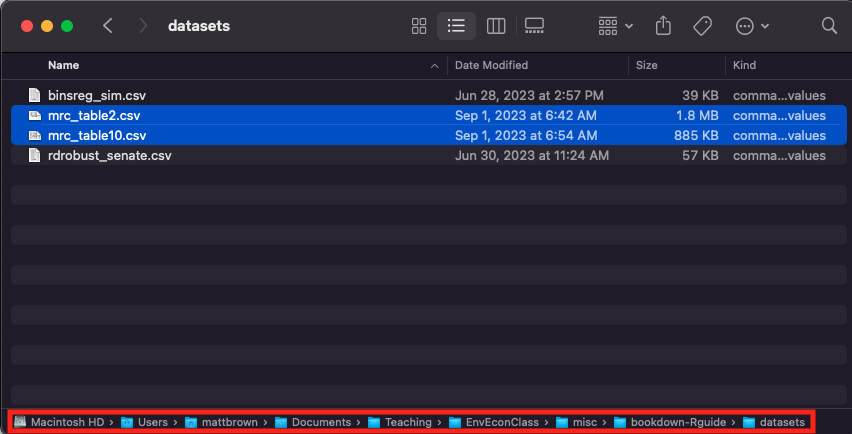
Figure 5.1: Datasets in a folder
If I wanted to access mrc_table2.csv, I could refer to the file’s exact location – that is, I could tell R to load /Users/mattbrown/Documents/Teaching/EnvEconClass/bookdown-Rguide/datasets/mrc_table2.csv. But that is a lot to type everytime I want to load a simple document.
Instead, I can tell R that this script “lives” in a folder called the working directory. Once I’ve done that, R treats the working directory as the highest-level folder. The following line sets the bookdown-Rguide/ folder as the working directory.
If you’re ever unsure what your working directory is, you can always ask R with getwd().
## [1] "/Users/mattbrown/Documents/Teaching/EnvEconClass/bookdown-Rguide"You can change your working directory either with the setwd() function or by using the RStudio “Session” tab. To set the working directory to the location of your Rscript (which is often desirable), click Session > Set Working Directory > To Sourcefile Location.
If you’re having trouble loading a dataset because of “no such file or directory” errors, it’s very likely that you have not set the working directory correctly, so this is a good first debugging step!
5.1.2 Reading csv files
Now that I’ve set the working directory, I can load the data files with the read.csv() function.10 The first data file contains the authors’ main mobility estimates, and the second contains supplemental variables from a dataset called the IPEDS Scorecard. I name the R objects accordingly.
5.2 Variable selection and subsetting
You can use names() to quickly glance at all the variables in your dataset.
##  [1] "super_opeid"          "name"                 "type"                 "tier"                 "tier_name"
##  [6] "iclevel"              "region"               "state"                "cz"                   "czname"
## [11] "cfips"                "county"               "multi"                "count"                "female"
## [16] "k_married"            "mr_kq5_pq1"           "mr_ktop1_pq1"         "par_mean"             "par_median"
## [21] "par_rank"             "par_q1"               "par_q2"               "par_q3"               "par_q4"
## [26] "par_q5"               "par_top10pc"          "par_top5pc"           "par_top1pc"           "par_toppt1pc"
## [31] "k_rank"               "k_mean"               "k_median"             "k_median_nozero"      "k_0inc"
## [36] "k_q1"                 "k_q2"                 "k_q3"                 "k_q4"                 "k_q5"
## [41] "k_top10pc"            "k_top5pc"             "k_top1pc"             "k_rank_cond_parq1"    "k_rank_cond_parq2"
## [46] "k_rank_cond_parq3"    "k_rank_cond_parq4"    "k_rank_cond_parq5"    "kq1_cond_parq1"       "kq2_cond_parq1"
## [51] "kq3_cond_parq1"       "kq4_cond_parq1"       "kq5_cond_parq1"       "kq1_cond_parq2"       "kq2_cond_parq2"
## [56] "kq3_cond_parq2"       "kq4_cond_parq2"       "kq5_cond_parq2"       "kq1_cond_parq3"       "kq2_cond_parq3"
## [61] "kq3_cond_parq3"       "kq4_cond_parq3"       "kq5_cond_parq3"       "kq1_cond_parq4"       "kq2_cond_parq4"
## [66] "kq3_cond_parq4"       "kq4_cond_parq4"       "kq5_cond_parq4"       "kq1_cond_parq5"       "kq2_cond_parq5"
## [71] "kq3_cond_parq5"       "kq4_cond_parq5"       "kq5_cond_parq5"       "ktop1pc_cond_parq1"   "ktop1pc_cond_parq2"
## [76] "ktop1pc_cond_parq3"   "ktop1pc_cond_parq4"   "ktop1pc_cond_parq5"   "k_married_cond_parq1" "k_married_cond_parq2"
## [81] "k_married_cond_parq3" "k_married_cond_parq4" "k_married_cond_parq5" "shareimputed"         "imputed"
That is a lot of variables! We don’t need to use most of them. The select() verb from the dplyr package lets us drop the variables we don’t need.
library(dplyr)
df_main = df_main %>%
  select(super_opeid, name, tier, mr_kq5_pq1, par_median, par_q1)
Let’s take this opportunity to review how dplyr verbs work.
- The object on the left of the
=operator is the new data.frame that will be created. In this case, we’re modifyingdf_main– so we’re saying, the “new”df_mainis equal to whatever comes to the right of the=. - The
%>%operator passes the left side object into the right side function as the first argument. All dplyr verbs, includingselect()take a data.frame as their first argument. This tellsselect()which data.frame it is working with. - The other arguments of
select()are variable names. The function returns a data.frame with only the variable names that you specify.
Let’s see how it works. We can look at df_main using the head() function, which prints the first five rows of a data.frame.
##   super_opeid                                            name tier mr_kq5_pq1 par_median     par_q1
## 1       30955 ASA Institute Of Business & Computer Technology   11 0.02003394      29000 0.44357517
## 2        3537                    Abilene Christian University    6 0.01436384     101000 0.05244136
## 3        1541            Abraham Baldwin Agricultural College    7 0.01485733      66000 0.15455516
## 4        7531                       Academy Of Art University   10 0.01635739      92300 0.09352423
## 5        1345                          Adams State University    5 0.01884468      67200 0.12922439
## 6        2666                              Adelphi University    6 0.03258507      96300 0.08704802
Now df_main only has a few variables! Mission accomplished.
select() lets us focus on specific variables (columns). What if we want to focus only on specific observations (rows)? Then we use the filter() verb.
As an example, let’s look atdf_IPEDS_Scorecard.
df_IPEDS_Scorecard = df_IPEDS_Scorecard %>%
  select(super_opeid, public, hbcu, flagship, scorecard_netprice_2013, state)
head(df_IPEDS_Scorecard)
## super_opeid public hbcu flagship scorecard_netprice_2013 state
## 1 30955 0 0 0 22011 NY
## 2 3537 0 0 0 20836 TX
## 3 1541 1 0 0 7887 GA
## 4 7531 0 0 0 28224 CA
## 5 1345 1 0 0 14705 CO
## 6 2666 0 0 0 20512 NYYou can see that there is a dummy variable for whether the institution is public. Let’s drop all non-public institutions. filter’s non dataframe arguments are logical statements in terms of the dataframe’s variables. filter() looks at all the statements you give it, checks its truth value each row, and drops all rows where any of the statements are false. Let’s see it in action.
##   super_opeid public hbcu flagship scorecard_netprice_2013 state
## 1        1541      1    0        0                    7887    GA
## 2        1345      1    0        0                   14705    CO
## 3        2860      1    0        0                    2810    NY
## 4       10056      1    0        0                    5315    SC
## 5        7582      1    0        0                    7958    CO
## 6        1002      1    1        0                   12683    AL
There we go! you can see that the non-public observations (about half of the rows) are now gone.
5.3 Merging datasets
We want to use the variables in df_main and df_IPEDS_Scorecard at the same time. They both describe the same univesities. How can we combine them? This is the analogy of the merge operation in STATA, but in dplyr the relevant function is called join.
The most important decision when joining dataframes is the key variable (or variables). Typically, the key will be a variable that identifies a unique observation in at least one dataset. In this case, we want to merge universities across the datasets. The super_opeid variable is a university id, so we will use it as the key.11
Let’s look at an example using the left_join() function, probably the most common type of join. You specify the key with the by option.
##   super_opeid                                            name tier mr_kq5_pq1 par_median     par_q1 public hbcu flagship
## 1       30955 ASA Institute Of Business & Computer Technology   11 0.02003394      29000 0.44357517     NA   NA       NA
## 2        3537                    Abilene Christian University    6 0.01436384     101000 0.05244136     NA   NA       NA
## 3        1541            Abraham Baldwin Agricultural College    7 0.01485733      66000 0.15455516      1    0        0
## 4        7531                       Academy Of Art University   10 0.01635739      92300 0.09352423     NA   NA       NA
## 5        1345                          Adams State University    5 0.01884468      67200 0.12922439      1    0        0
## 6        2666                              Adelphi University    6 0.03258507      96300 0.08704802     NA   NA       NA
##   scorecard_netprice_2013 state
## 1                      NA  <NA>
## 2                      NA  <NA>
## 3                    7887    GA
## 4                      NA  <NA>
## 5                   14705    CO
## 6                      NA  <NA>
You can see that the data.frame now has the variables from both the left argument df_main and the right argument df_IPEDS_Scorecard. The vales for the df_main variables are exactly the same as before, and the values for the df_IPEDS_Scorecard variables are the ones that belong to the university with the matching super_opeid. This is what left_join() does. It starts with the left-side data.frame and then looks for matching cases on the right side to fill in the values for the right-side variables.
Note that we did not succeed in matching all of the observations from df_main matched – some of the observations have NA values for the right-side variables. This should not be surprising. We dropped all non-public institutions from the right-side data, so no matches existed for the non-public variables in df_main.
It is sometimes convenient to use a join that automatically drops all these cases where the left side and right side do not match. inner_join() accomplishes this.
##   super_opeid                                            name tier mr_kq5_pq1 par_median     par_q1
## 1       30955 ASA Institute Of Business & Computer Technology   11 0.02003394      29000 0.44357517
## 2        3537                    Abilene Christian University    6 0.01436384     101000 0.05244136
## 3        1541            Abraham Baldwin Agricultural College    7 0.01485733      66000 0.15455516
## 4        7531                       Academy Of Art University   10 0.01635739      92300 0.09352423
## 5        1345                          Adams State University    5 0.01884468      67200 0.12922439
## 6        2666                              Adelphi University    6 0.03258507      96300 0.08704802
Note that df_main now only has public institutions. This is because the non-public institutions don’t appear in the (filtered) df_IPEDS_Scorecard, so they were dropped.
5.4 Pausing to look at the data
It’s typically a good idea to look at your own data every now and then as you are cleaning it, and certainly before you implement any formal analyses. One quick way to make a summary table of numeric variables is to use the datasummary_skim package from modelsummary.
library(modelsummary)
df_to_summarize = df_main %>% select(par_median, mr_kq5_pq1, par_q1)
datasummary_skim(df_to_summarize)| Unique | Missing Pct. | Mean | SD | Min | Median | Max | Histogram | |
|---|---|---|---|---|---|---|---|---|
| par_median | 911 | 0 | 77695.5 | 28463.3 | 21200.0 | 74300.0 | 226700.0 |  |
| mr_kq5_pq1 | 2188 | 0 | 0.0 | 0.0 | 0.0 | 0.0 | 0.2 |  |
| par_q1 | 2202 | 0 | 0.1 | 0.1 | 0.0 | 0.1 | 0.6 |  |
That function automatically creates a rough summary table for your variables. You can also use the more customizable datasummary() function – see documentation here. Following that documentation, here is some sample code that makes a table that also includes the number of observations.
| Mean | Median | P100 | P0 | N | |
|---|---|---|---|---|---|
| par_median | 77695.46 | 74300.00 | 226700.00 | 21200.00 | 2202 |
It’s also helpful to visualize your data graphically. Plotting can give you an intuitive understanding of your data. It can also highlight strange features that you might have missed previously – you can ask, “does this data pass the smell test?” For example, let’s start with a histogram.12
library(ggplot2)
hist_price = ggplot(data = df_merged, aes(x = scorecard_netprice_2013)) +
    geom_histogram()

hist_price
## `stat_bin()` using `bins = 30`. Pick better value with `binwidth`.## Warning: Removed 1 row containing non-finite outside the scale range (`stat_bin()`).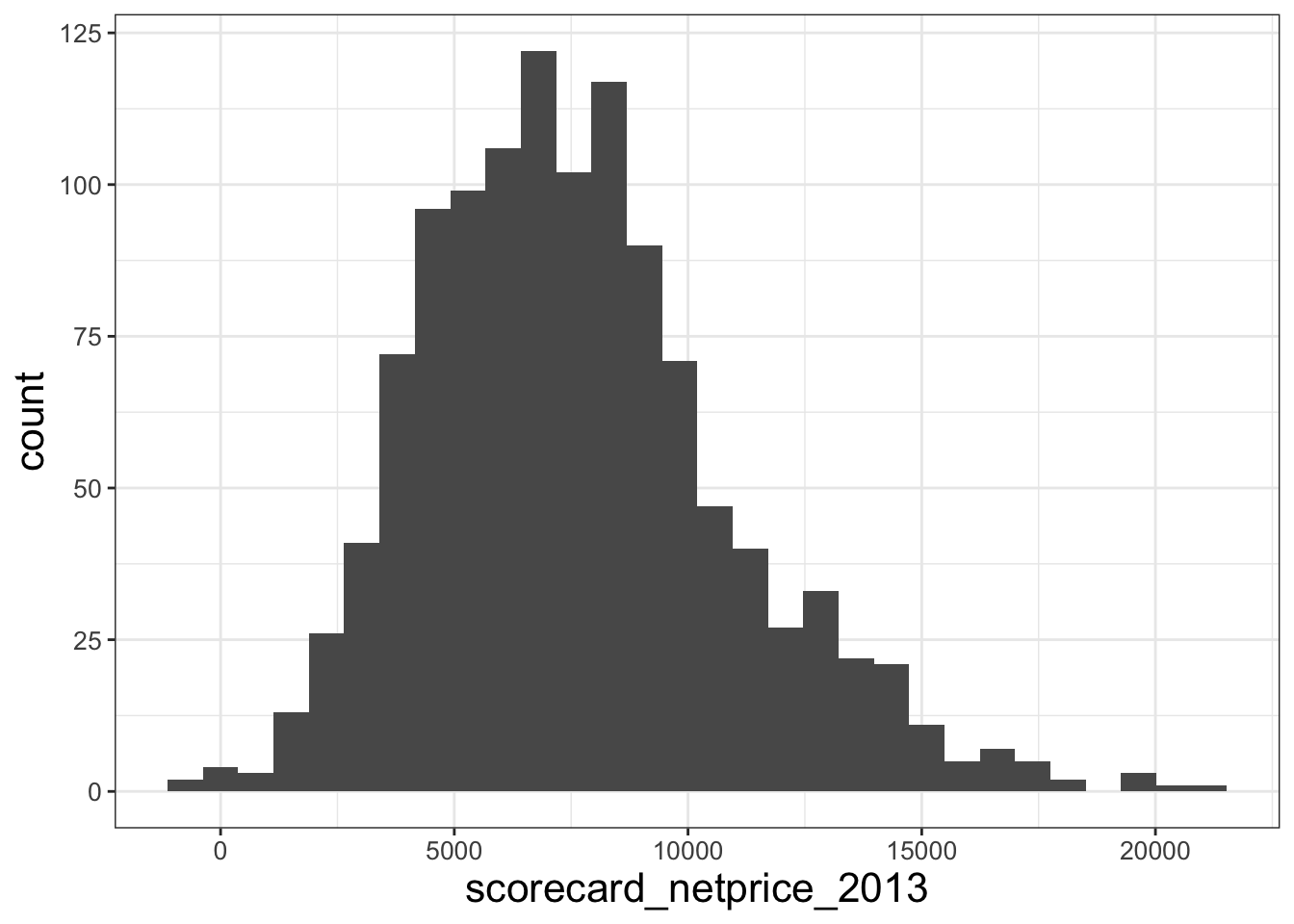
5.4.1 Dealing with outliers and missing values
Examine that last histogram. The histogram for scorecard_netprice_2013 has some negative values. Is it true the the average net price of college attendance for students from the bottom 20% of the income distribution is negative at some public schools?
Let’s look at the observations that have negative prices.
##   super_opeid                                                        name tier mr_kq5_pq1 par_median    par_q1 public hbcu flagship
## 1        8082                                 Cleveland Community College    9 0.01453786      49600 0.2031542      1    0        0
## 2        1073                                     Eastern Arizona College    9 0.02299221      60900 0.1434419      1    0        0
## 3        1742 Illinois Eastern Community Colleges - Olney Central College    9 0.01368477      58400 0.1687605      1    0        0
##   scorecard_netprice_2013 state
## 1                     -58    NC
## 2                   -1071    AZ
## 3                    -955    IL
These are three small community colleges with low sticker prices. It seems plausible that students recieving aid and scholarships could receive a negative price to attend. But let’s do some more digging. It turns out that on the College Scorecard website, which was the source of this data, they explicitly mention that an institution might have a negative net price: “Negative cost values indicate that the average grant/scholarship aid exceeded the cost of attendance.” So I take the values literally and I do not drop them.
Sometimes, it’s the right course of action to keep outliers. Other times, it’s better to drop them. In general, you want to drop outliers that you think are data errors, and you might want to include outliers if the data correspond to true values in your population of interest.
Now let’s talk about what to do with missing values in the data. Note that with the current dataset, if I try to compute the average price with the mean() function, R will not give me a number.
## [1] NAThis is because there are observations with missing price data. By default, R stores missing data as NA. Let’s look at the observations with missing prices.
##   super_opeid                          name tier mr_kq5_pq1 par_median    par_q1 public hbcu flagship scorecard_netprice_2013 state
## 1       21922 Thomas A Edison State College    7 0.04188218      79300 0.1035151      1    0        0                      NA    NJ
These colleges just don’t have data on attendance prices. Since I’m going to be analyzing the correlation between price and mobility, I remvove them from the dataset.13
5.5 Summarizing and grouped operations
5.5.1 summarize()
The next dplyr verb is summarize(). summarize accepts as inputs functions of variables in the dataset that you specify. The functions that you specify should take several observations and summarize them in one number – for example, computing a mean or a median.14 Here is one example
df_merged %>% summarize(
  avg_price = mean(scorecard_netprice_2013), #Summary function 1
  fraction_in_CA = mean(state=='CA') # summary function 2
)
## avg_price fraction_in_CA
## 1 7616.552 0.08410429Unlike with previous verbs, the output is not a data.frame of the same shape as the input data.frame. Instead, summarize() returns a dataset with only one observation (!) and the values of your chosen summary functions as variables. In this case, the output tells us that the average price across public colleges is $7616, and 8.4% of the colleges in the data are in California.
Often, you’ll want to compute the same statistics for several variables at once. But it’s tedious to type out mean(x1), mean(x2), mean(x3) when you have many xs. Instead, use a shortcut: summarize(across()).
df_merged %>%
  summarize(across(
    c(mr_kq5_pq1, scorecard_netprice_2013),
    list('med' = median, 'avg' = mean)
  ))
## mr_kq5_pq1_med mr_kq5_pq1_avg scorecard_netprice_2013_med scorecard_netprice_2013_avg
## 1 0.01582546 0.01914963 7213 7616.552across() is a function that you can only call inside a dplyr verb.15. You use it when you want to manipulate several variables in the same way. The first input to across() specifies the variables you want to manipulate, and the second input specifies the desired manipulations. When you want to make multiple manipulations, you use a named list to tell R what the output variables should look like. For example, above, I am telling R to put _med at the end of the variable name to designate the median computations.
5.5.2 Pivoting
Sometimes (e.g, on the IncomePollutionHealth problem set), we want to take the output of summarize() and reorganize it into a presentable table.16 The problem is that the table above is hard to read – it’d be better if, say each statistic was a row, and each variable was a column, so you could quickly look up any values you need. This is a case where we have already computed the values we need, but we need to change the shape of the data. The need to change rows into columns comes up fairly often in larger projects – it may arise for in your E3 paper! The standard approach is to use pivot_ functions from the tidyverse package.17
A full description of how pivot_ works is beyond scope for this guide. And frankly, I always have to re-lookup the documentation anyways when I start reshaping. For details, start with this online vignette. Here, I provide sample code for reshaping summary outputs into cleaner tables.
library(tidyverse)
# Reshape summary table with pivot_longer()
df_table = df_merged %>%
  summarize(across(
    c(mr_kq5_pq1, scorecard_netprice_2013),
    list('stat_median' = median, 'stat_mean' = mean)
  )) %>%
  pivot_longer(
    everything(), # Tells R: Use all columns!
    names_sep = '_stat_', # Tells R: the variables are named so that the name of
    # the summary stat always comes after the string "_stat_", and the variable
    # we are summarizing comes before that string..
    names_to = c('.value', 'statistic'), # Tells R: store the summary statistic
    # variable in a new column called "statistic".
    )
If you’d prefer to switch the rows and columns of your table – well, there’s also a way to do that with pivot functions!
df_table = df_table %>%
  pivot_longer(cols=c(-statistic), names_to="Original_Vars") %>%
  pivot_wider(names_from=c(statistic))
print(df_table)
## # A tibble: 2 × 3
## Original_Vars median mean
## <chr> <dbl> <dbl>
## 1 mr_kq5_pq1 0.0158 0.0191
## 2 scorecard_netprice_2013 7213 7617.Again, I advise looking at the documentation.
5.5.3 Grouped summarize
summarize() really shows its power when combined with another dplyr verg, group_by(). Here’s how I think about group_by(). It doesn’t do anything to a dataset by itself. Instead, if you write df %>% group_by(var), you are planting a flag in the df that tells R: “If you ever compute a summary statistic for df, you should compute the summary statistic separately for each unique level of var.”
Here’s an example with summarize.
df_merged %>% group_by(hbcu) %>%
  summarize(across(
    c(mr_kq5_pq1, scorecard_netprice_2013),
    list('median' = median, 'mean' = mean)
  ))
## # A tibble: 2 × 5
## hbcu mr_kq5_pq1_median mr_kq5_pq1_mean scorecard_netprice_2013_median scorecard_netprice_2013_mean
## <int> <dbl> <dbl> <dbl> <dbl>
## 1 0 0.0156 0.0188 7184 7548.
## 2 1 0.0289 0.0290 9408 9799.You can see that we’ve now computed summary statistics separately for HBCUs and other universities! Each group gets its own row.
You can also group_by multiple variables. That will make a separate row for each unique combination of group variables that exists in the data. I give an example of that below. The example also illustrates the use ofthe n summary function, which just counts the number of observations in the group.18
df_counts = df_merged %>% group_by(state, hbcu) %>%
  summarize('avg_mobility' = mean(mr_kq5_pq1), 'n' = n())
head(df_counts)
## # A tibble: 6 × 4
## # Groups: state [4]
## state hbcu avg_mobility n
## <chr> <int> <dbl> <int>
## 1 AK 0 0.0154 1
## 2 AL 0 0.0201 27
## 3 AL 1 0.0269 5
## 4 AR 0 0.0190 27
## 5 AR 1 0.0283 1
## 6 AZ 0 0.0193 11Looking at the second and third rows, last column tells us that the data contains 27 non-HBCUs from Alabama. and 5 HBCUs. Note that there is no hbcu=1 row for Alaska. This is because the data does not contain any Alaska HBCUs.
5.6 Common variable manipulations
Here are some common types of new variables that you might create.
5.6.1 Indicator variables
We often want to make a variable that takes value 1 if a condition is true, and 0 otherwise. Recall from Section 3 that as.numeric() converts logical values to zeros and ones. So one way to make an indicator variables is to use code like this: df = df %>% mutate(indicator = as.numeric(condition)). Here’s an example
df_merged = df_merged %>%
  mutate(par_median_above_100K = as.numeric(par_median > 100000))
print(mean(df_merged$par_median_above_100K))
## [1] 0.07401177So 7.4% of colleges in the sample have parental median income over $100,000.
5.6.2 Factors
A categorical variable is a variable that can only take one of a number of fixed values. For example, state in the current dataset is a categorical variable in the sense that it can only take one of 51 values (50 states + DC). You’ll never see state take value 'Tatooine' or 5343232. By contrast, character and numerical values have no such limits on their possible values.
Sometimes, it’s useful to explicitly tell R to store some variables as categorical variables. R calls categorical variable “factors” (see here). Describing factors is beyond scope for this guide. I only provide sample code below for creating a factor.
df_IPEDS_Scorecard = df_IPEDS_Scorecard %>% mutate(f.state = factor(state))
print(df_IPEDS_Scorecard$state[1:10])
## [1] "GA" "CO" "NY" "SC" "CO" "AL" "AL" "AL" "NC" "TX"## [1] GA CO NY SC CO AL AL AL NC TX
## 51 Levels: AK AL AR AZ CA CO CT DC DE FL GA HI IA ID IL IN KS KY LA MA MD ME MI MN MO MS MT NC ND NE NH NJ NM NV NY OH OK OR PA ... WYI will flag that I have found creating factor variables useful when plotting. This is because factors have tools that allow you to define the order of potential values (so-called “levels” of the factors). By controlling the level orders, you can control the order of variables on the axes of your plots.
5.6.3 Group averages
Just as group_by interacts with summarize, it also interacts with mutate. If you group a dataset before passing it into mutate, and then give mutate a summary statistic function, R computes the summary statistic at the group level for each variable. Here is an example/
df_merged = df_merged %>%
  mutate(ovr_avg_mobility = mean(mr_kq5_pq1)) %>%
  group_by(hbcu) %>%
  mutate(type_avg_mobility = mean(mr_kq5_pq1)) %>%
  ungroup()
print(head(df_merged %>% select(hbcu, ovr_avg_mobility, type_avg_mobility)))
## # A tibble: 6 × 3
## hbcu ovr_avg_mobility type_avg_mobility
## <int> <dbl> <dbl>
## 1 0 0.0191 0.0188
## 2 0 0.0191 0.0188
## 3 0 0.0191 0.0188
## 4 0 0.0191 0.0188
## 5 1 0.0191 0.0290
## 6 0 0.0191 0.0188You can see that before I group the data, mutate computes an average across the dataset as a whole. But after grouping, mutate makes group averages.
Note that at the end of this chain I make sure to pass the data.frame through ungroup(), to ensure that I don’t inadverdently start working with a grouped data.frame next time I manipulate df_merged.
The data is stored at the Opportunity Insights website.
mrc_table2.csvis the file “Baseline Cross-Sectional Estimates of Child and Parent Income Distributions by College.”mrc_table10.csvis the file “College Level Characteristics from the IPEDS Database and the College Scorecard.”↩︎This function can slow for large datasets.
freadandvroomare two alternatives to load large datasets locally. If your dataset is not in a .csv format, you’ll need a different function.↩︎If you don’t specify a key yourself, R will automatically assume that any variables that share the same name across both datasets are keys. Sometimes this is desirable, but sometimes it’s not – in general, you want to make sure you’re clear about what the key is.↩︎
Scatter plots and binscatters are also useful plots to make while cleaning.↩︎
You can also use the
drop_na()function in thetidyversepackage to drop observations with missing values in any column. However, I don’t necessarily recommend this course of action, since you don’t always know why certain observations are being dropped. Much better to understand, for each variable with missing values, why the values are missing, and what dropping them means for your analysis.↩︎See documentation for a list of some helpful functions.↩︎
See documentation and a vignette↩︎
An alternative for table creation is the
datasummaryfunction inmodelsummarypackage (documentation), which creates tables like the ones you made withdatasummary_skim(). Documentation here. I likedatasummarya lot, but others find it confusing. It’s a matter of taste.↩︎The
pivot_functions are the analogy of thereshapecommand in Stata.↩︎count()is also shorthand forsummarize(n()). So you can dodf_merged %>% group_by(state) %>% count()to quickly count the number of observations in each state, for example. Very helpful in the early stages of cleaning!↩︎