4 Results

4.1 Coverage

4.1.1 Geographical coverage

Should probably include a map here of the countries that we have included. Here is a list instead to start with

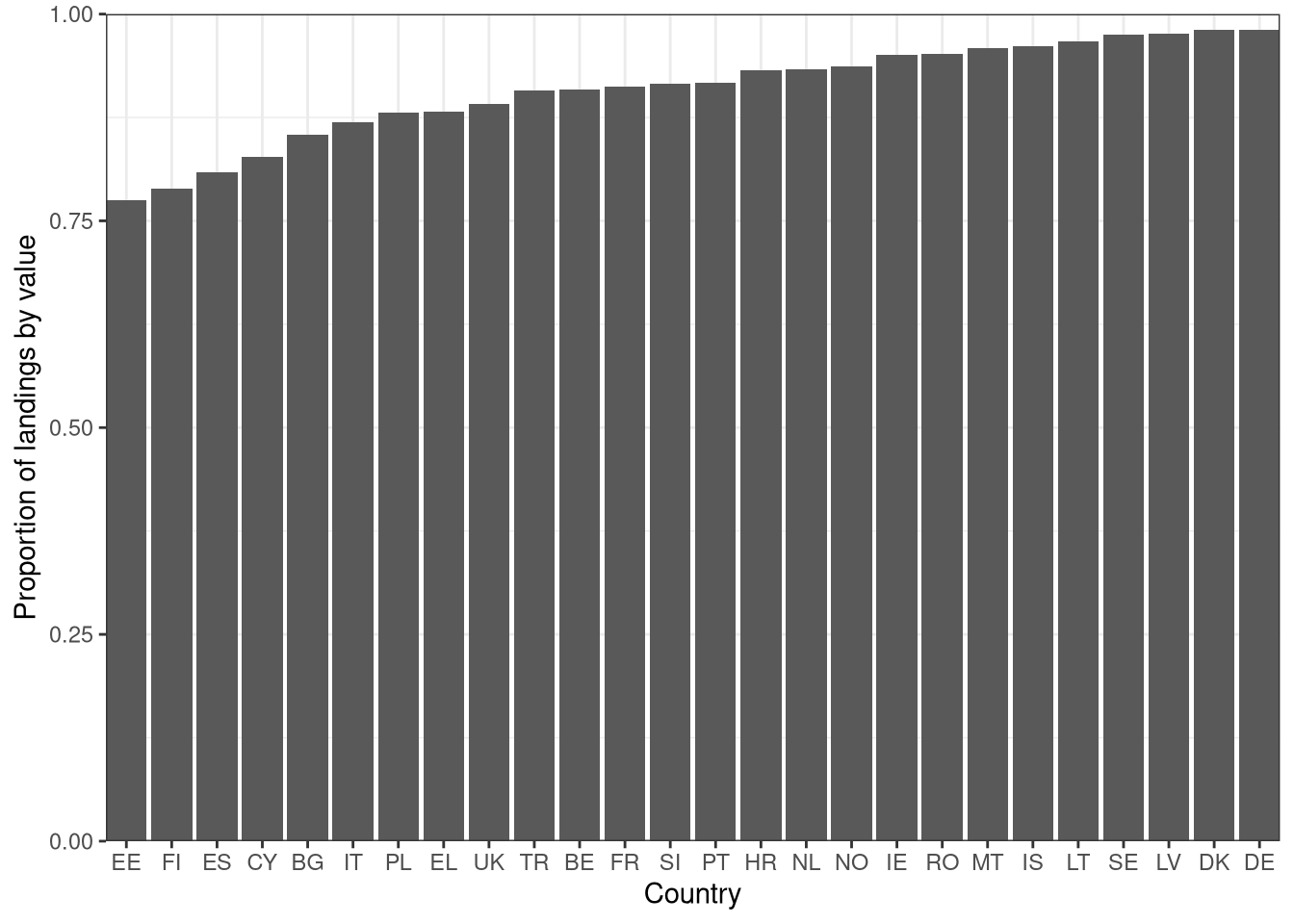
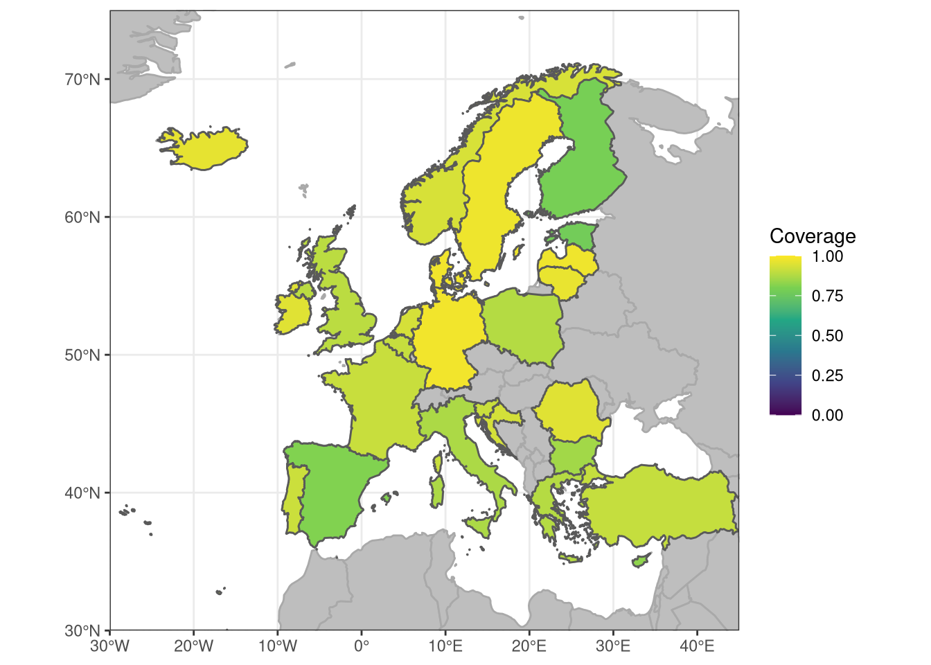
A complete set of trait and Aquamap data (allowing the calculation of climate hazard) was gathered for 147 species caught in European waters, representing 90.3% of the total value of fish and shellfish landings in Europe. Catch data was available covering 26 countries in Europe: country-wise coverage was at least 78% by value and typically above 90%.

When combined with catch data covering 23 FAO subareas, this resulted in a total of 1300 potential “stocks”. However, many of these stocks made relatively minor contributions to the total catch of the species: stocks comprising less than 5% of the total catch of that species were therefore filtered out, leaving 523 stocks in the analysis.

4.1.2 Fleet Coverage

We should also check the coverage by fleet segment. We are able to do the full analysis for 404 fleet segments, although the coverage of some of these units can be pretty poor.

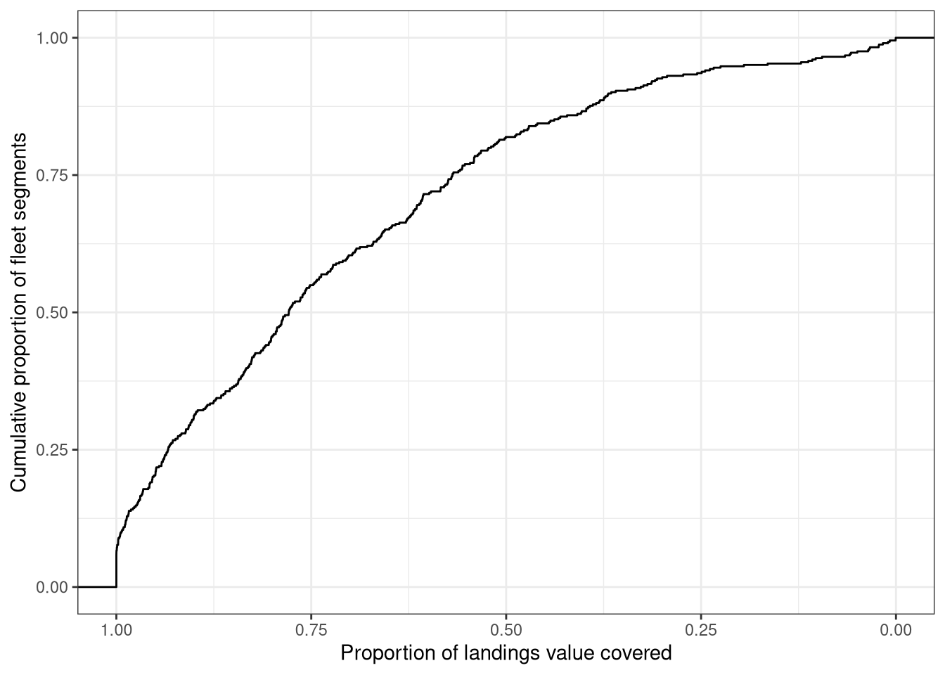
Nevertheless, we still cover 75% or more of the landings value for more than 70% of fleets. We should probably filter this at some point to focus on the most important and/or best covered fleets.

Number of fleet segements: 358

4.2 Biological metrics

4.2.1 Species-specific metrics

As a cross check that we have implemented the coversion from these metrics to a hazard, we plot one against the other, to ensure that the trend is as intended

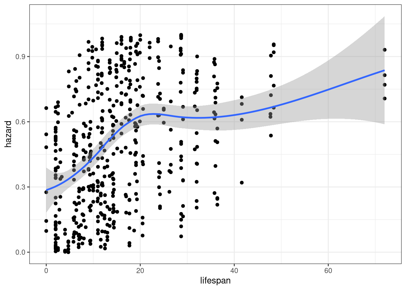
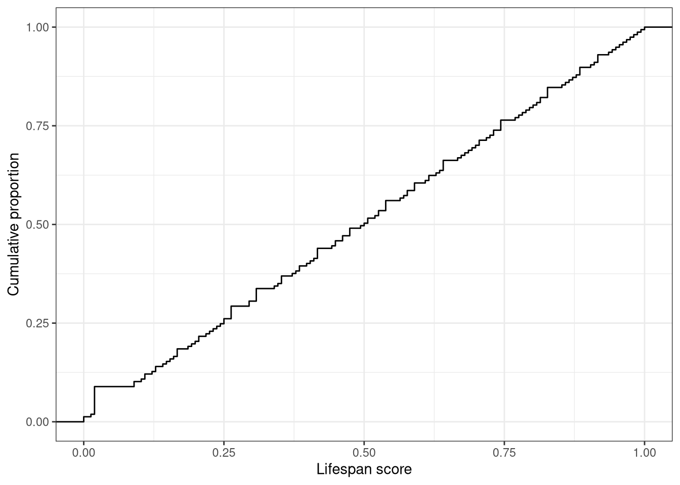
So, longer-lived species have a higher hazard score. Tick.

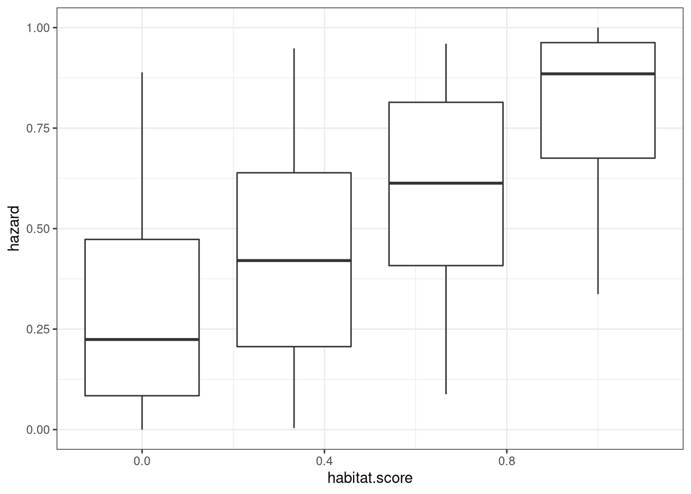
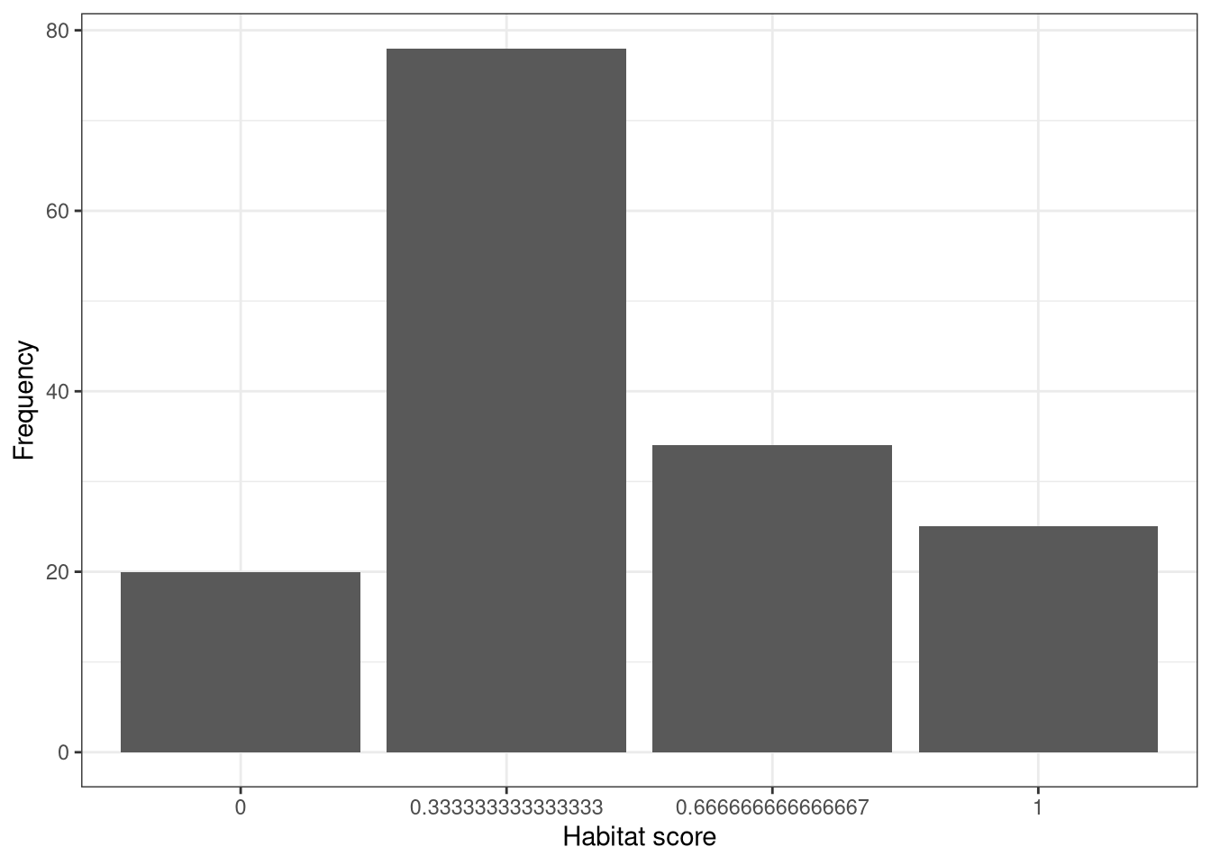
So species with a higher habitat-specificity have a higher hazard. Tick.

4.2.2 Stock-specific metrics

Small stocks are a potential problem in this analysis. We first check the distribution of stock sizes (expressed as value of landings) relative to the total size (value) of the species.

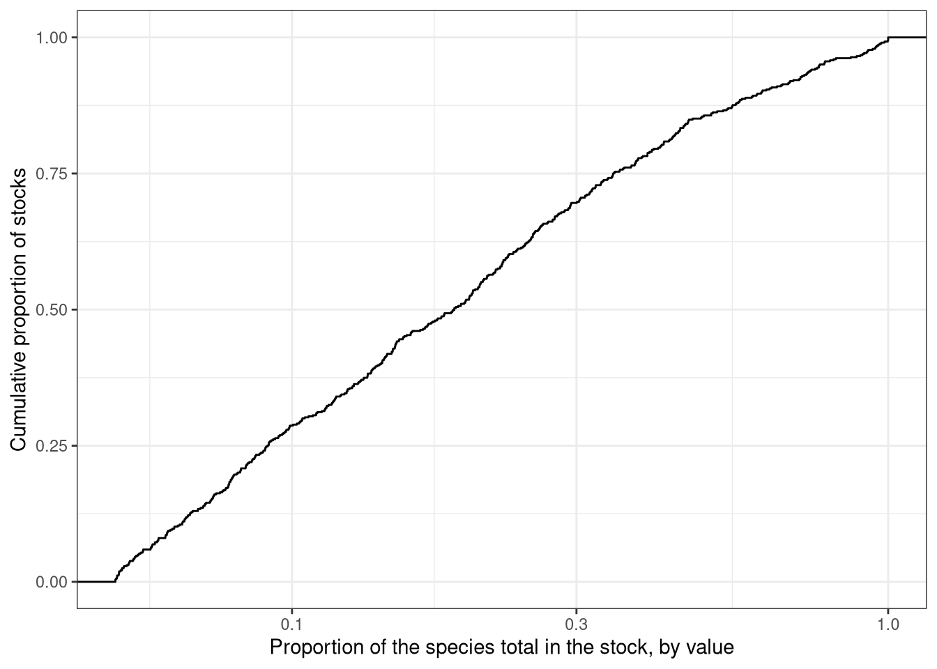
We can therefore see that there are an awful lot of stocks that don’t contribute much landigns value - is is a natural consequence of the way that we have defined a stock in this case. We choose to filter out all stocks that have a landings value less than 5% of the species total.

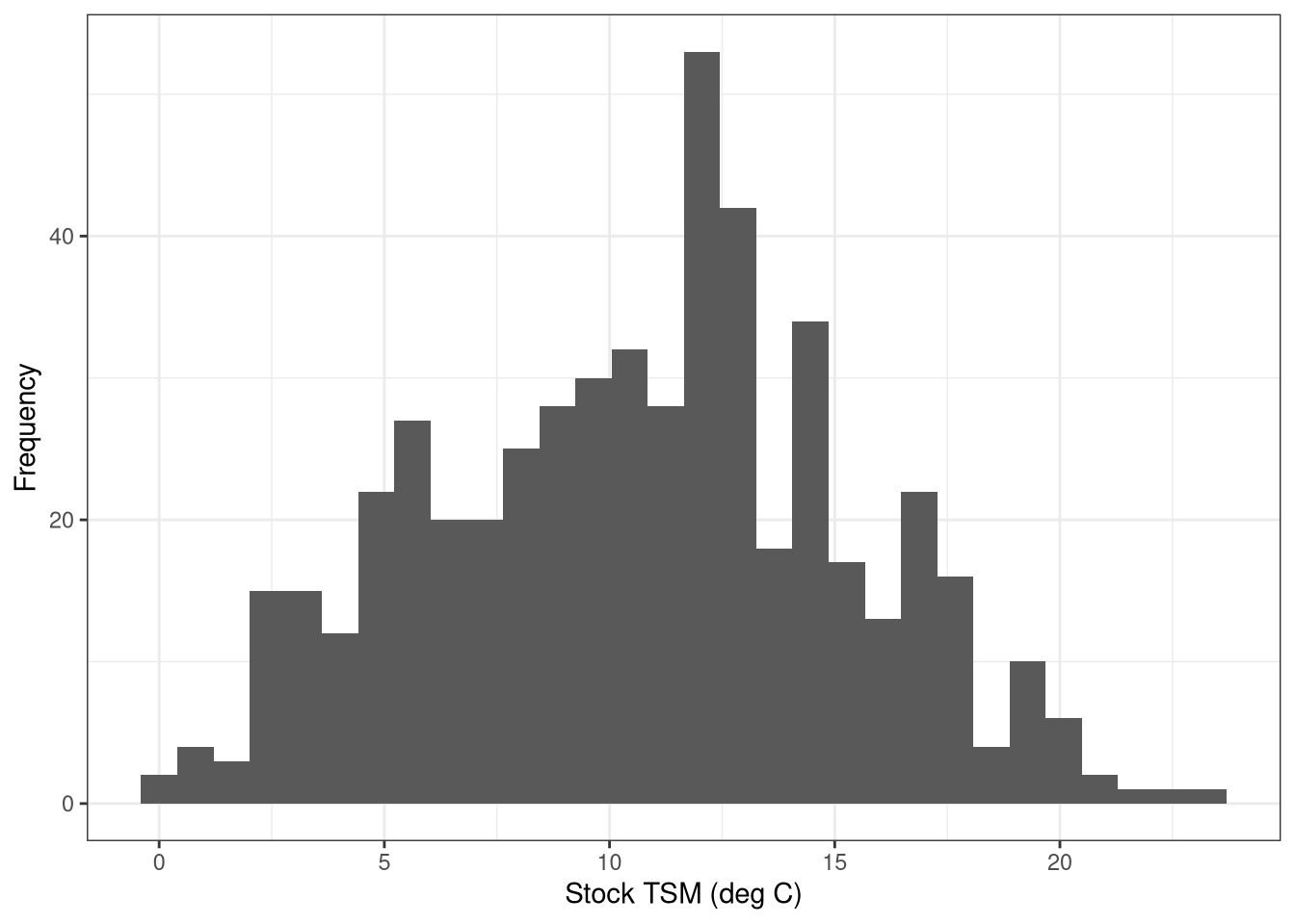
This leaves us with 523 stocks. Looking at the distribution of TSM’s of these remaining stocks.

And cross checking the hazard implementation.

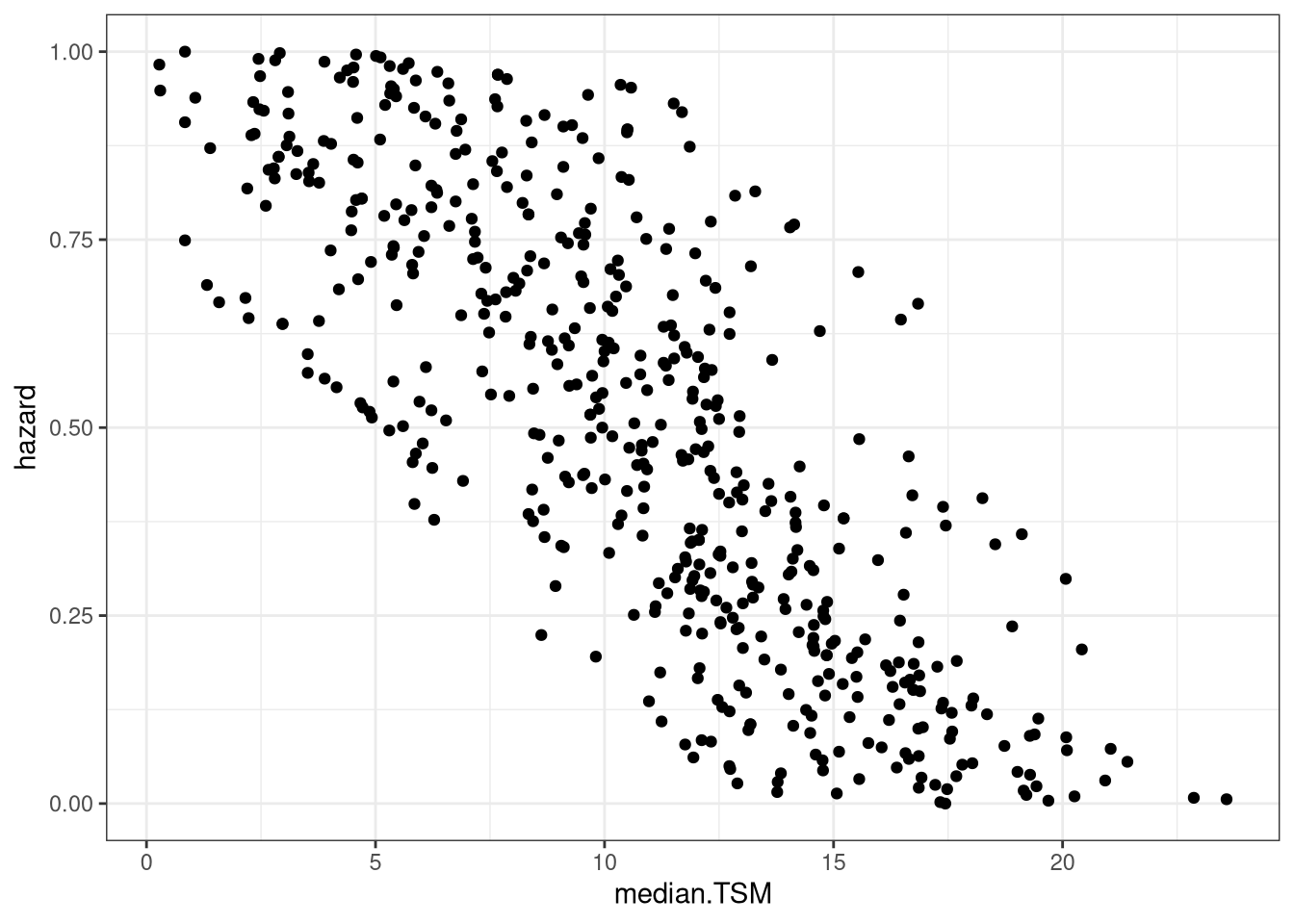
Low TSMs => higher hazards. Tick. The stripping rises due to the categorical natural of the other metrics.

4.2.3 Species-level hazard

We can look at our biological analysis by integrating the hazard back up to the species level by weighting by the value of landings of each stock.

Looking at the top and bottom ten species

FAO_3A_code	FAO_EN	hazard	rank
WHE	Whelk	0.8828335	1
DEC	Common dentex	0.8790946	2
KLK	Smooth callista	0.8434970	3
FOR	Forkbeard	0.7948277	4
OYF	European flat oyster	0.7771141	5
SCE	Great Atlantic scallop	0.7704106	6
HKX	Hakes nei	0.7291516	7
PRR	Parrotfish	0.7263368	8
SVE	Striped venus	0.7242199	9
MEG	Megrim	0.7199062	10
OCC	Common octopus	0.2299293	139
HER	Atlantic herring	0.2271872	140
SQI	Northern shortfin squid	0.2237962	141
SPR	European sprat	0.2159665	142
SQC	Common squids nei	0.2020260	143
SQM	Broadtail shortfin squid	0.1988565	144
OCZ	Octopuses nei	0.1905851	145
BLT	Bullet tuna	0.1679663	146
SSH	Scarlet shrimp	0.1310705	147
BON	Atlantic bonito	0.1093046	148

4.3 Fleet metrics

4.3.1 Fleet hazard metrics

Fleets with the top and bottom 10 hazard scores

Table 1: Top and botton 10 fleets by hazard

fs_name	value.covered	total.val.landings	prop.missing	hazard
EST A27 TM1218	860437.0	860437.0	0.0000000	0.0550035
LTU A27 TM2440 °	13475876.0	13475876.0	0.0000000	0.0588392
EST A27 TM2440 °	48072014.0	48072264.0	0.0000052	0.0627536
POL A27 TM2440 °	73972680.3	75163367.3	0.0158413	0.0677118
FIN A27 TM2440 °	107055789.0	107065174.7	0.0000877	0.0704230
FIN A27 TM1824	30019850.0	30019850.0	0.0000000	0.0705229
FIN A27 TM1218 °	10807913.8	10983806.6	0.0160138	0.0742556
EST A27 PG1012	7613725.0	7630744.0	0.0022303	0.0761999
PRT A27 FPO0010	1681210.0	1741082.0	0.0343878	0.0825611
PRT A27 FPO1012	1086829.0	1139708.0	0.0463970	0.0863356
BEL A27 PMP1824 °	473171.6	495884.6	0.0458029	0.8846257
FRA A27 DRB0010	1406833.8	8547518.7	0.8354103	0.8850338
GBR A27 DRB0010	2022678.0	2657277.3	0.2388156	0.8903896
FRA A27 FPO1012	8163528.9	8435296.8	0.0322179	0.8913679
IRL A27 FPO0010	4408690.9	5406757.3	0.1845961	0.9163961
ESP A27 DRB1012	291963.2	293883.4	0.0065339	0.9236067
ESP A27 DRB1218	2284353.2	2285575.2	0.0005347	0.9291188
GBR A27 DRB1012	1972195.2	2077496.5	0.0506866	0.9356896
IRL A27 DRB2440 °	2004905.0	2004905.0	0.0000000	0.9635988
ITA A37 DRB1218 °	17394834.4	17772573.7	0.0212541	0.9687215

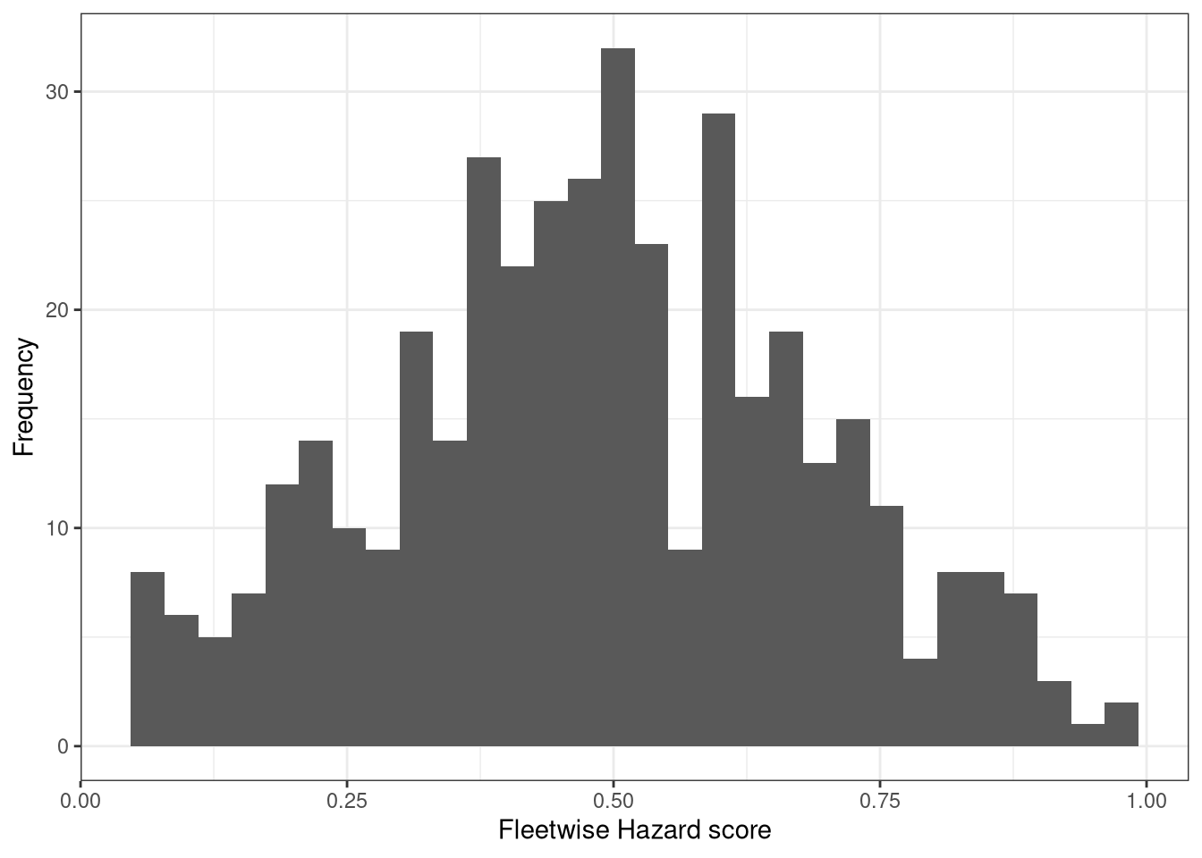
Figure 6: Distribution of hazard metrics

4.3.2 Fleet exposure metrics

We use the Shannon diversity and the Simpson Dominance metrics to characterise the diversity of species that a fishing fleet catching. The distribution of these metrics is as follows.

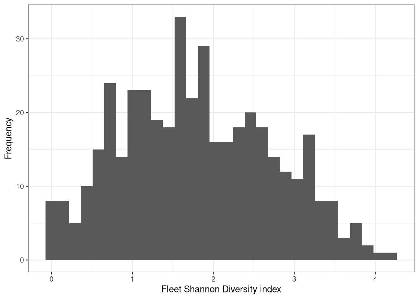
Figure 7: Fleetwsie Shannon Diversity index

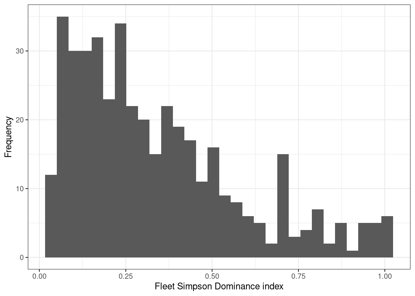
Figure 8: Fleetwise Simpson Dominance

A correlation between these two metrics is expected.

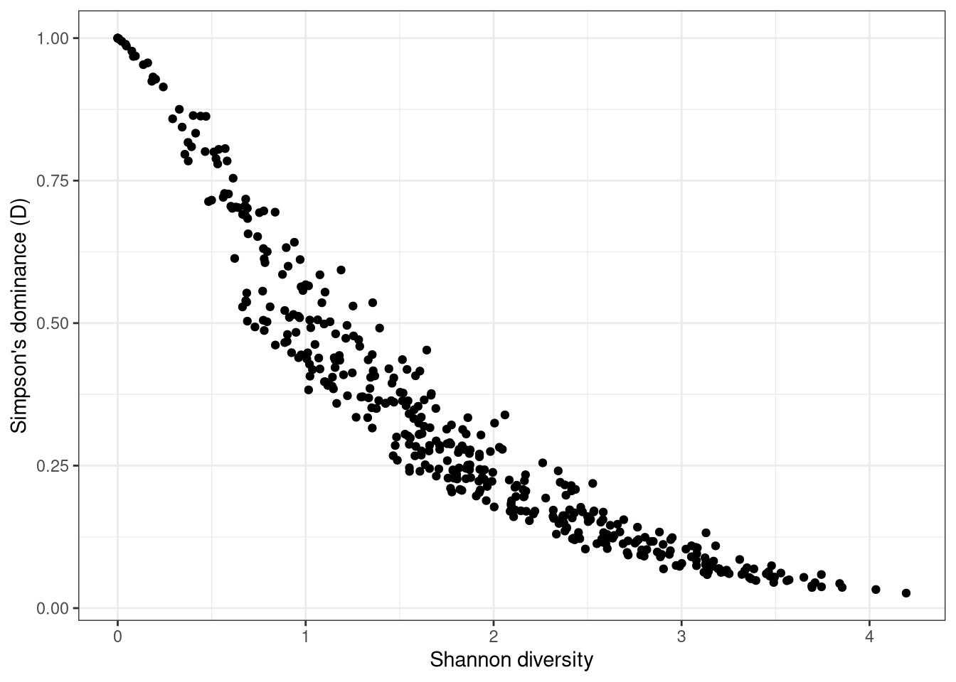
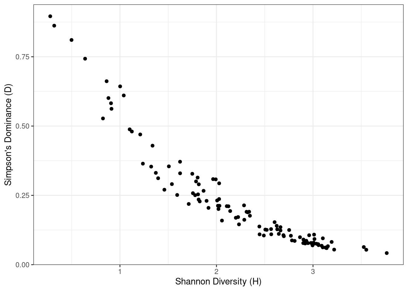
Figure 9: Relationship between Shannon Diversity H’ and Simpson’s Dominance D of fishery landings, for EU fleet segments in 2016

Clearly there is a strong relationship between Shannon diversity of fishery landings and Simpson’s dominance (D), although this is not linear (figure 1).

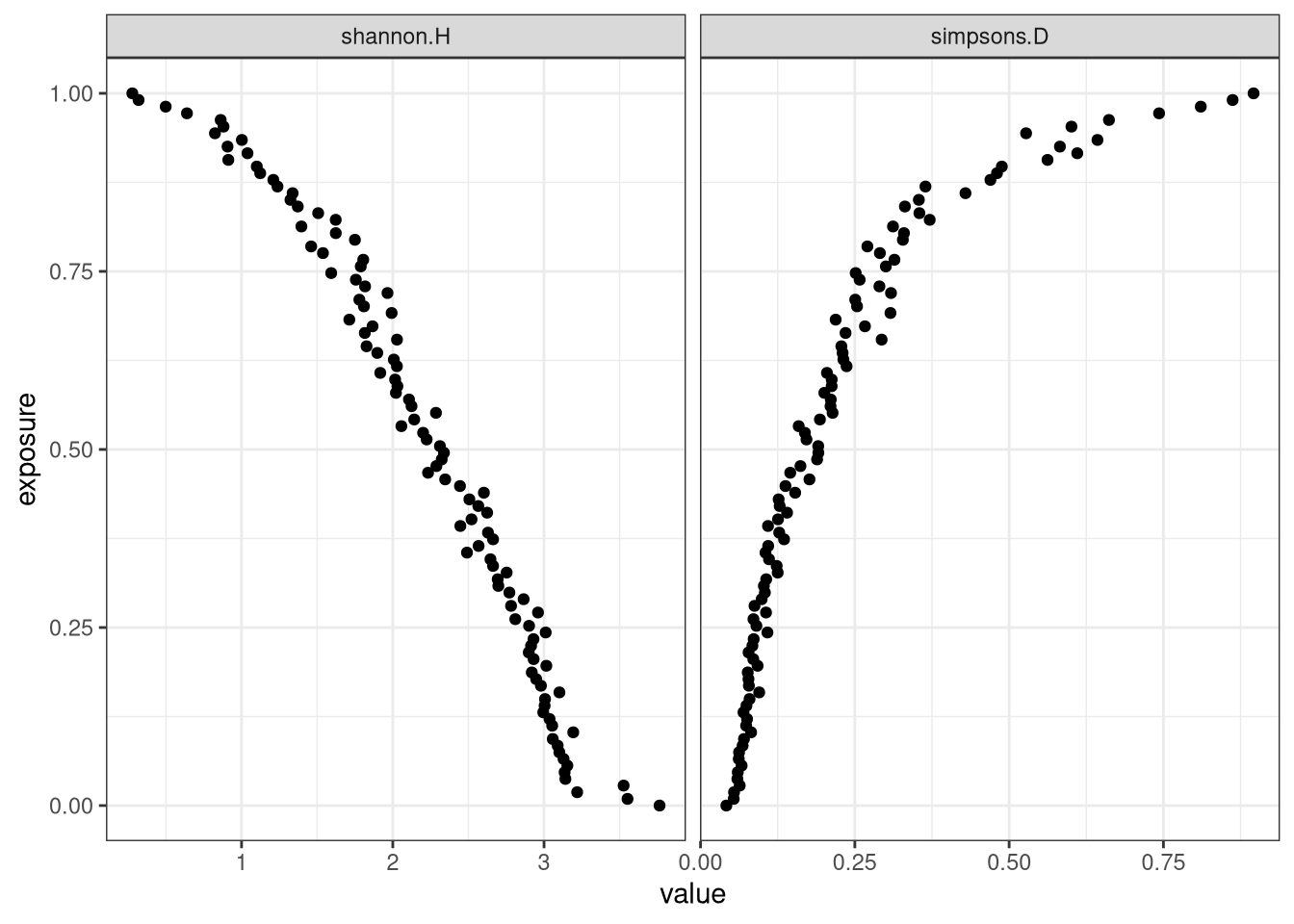
We combine the two metrics together into a into exposure metrics. Checking that we have done this correctly:

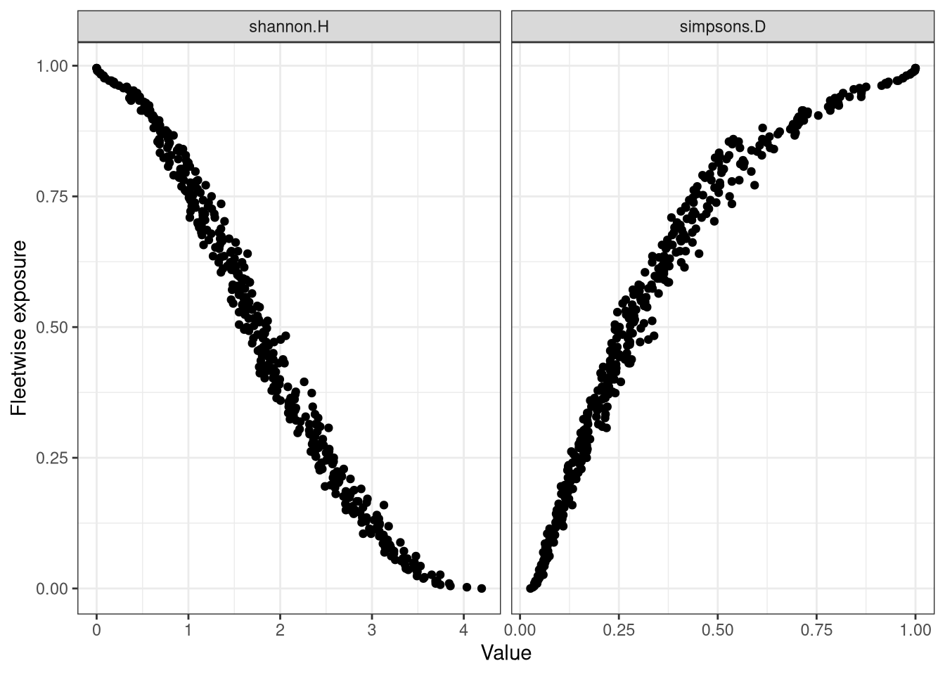
Figure 10: Exposure vs Shannon Index

So fleets with higher diversity have lower exposure. Tick. And fleets that are dominated by a few species have a higher exposure, which is what we want.

Plotting the list of fleet diversity.

Least diverse fleets

Table 2: Least diverse fleets

fs_name	sum.prop	sum.value	shannon.H	simpsons.D	n.species	exposure
IRL A27 DRB2440 °	1	2004905	0.0000000	1.0000000	1	0.9952381
MLT A37 PS2440	1	360500	0.0000000	1.0000000	1	0.9952381
PRT A37 FPO2440	1	116207	0.0000000	1.0000000	1	0.9952381
ESP A27 DRB1218	1	2285575	0.0049305	0.9989311	3	0.9928571
DEU A27 TBB1012 °	1	61863	0.0058449	0.9986430	3	0.9904762
ROU A37 PMP1218 °	1	4157697	0.0214070	0.9944113	10	0.9880952

Most diverse fleets

Table 3: Most diverse fleets

fs_name	sum.prop	sum.value	shannon.H	simpsons.D	n.species	exposure
ESP A37 PMP0612	1	4814591	3.743704	0.0589389	347	0.0261905
FRA A37 DFN0612	1	1337565	3.744439	0.0373679	203	0.0071429
ESP A37 DTS2440	1	5647283	3.841203	0.0431922	476	0.0095238
ITA A37 PGP0612	1	21059018	3.854408	0.0363553	135	0.0047619
ESP A37 DTS1218	1	4437824	4.033915	0.0326257	701	0.0023810
ESP A37 DTS1824	1	11824853	4.194966	0.0263463	746	0.0000000

Catch diversity in 2016 ranged from zero (where a fleet caught a single resource) to 4.19, where a multitude of different fish and shellfish species were targeted. The lowest diversity of catches was observed for the fleet segments IRL-A27-DRB2440, MLT-A37-PS2440 and PRT-A37-FPO2440, fishing exclusively on Great Atlantic scallop (Pecten maximus), Chub mackerel (Scomber colias) and Striped soldier shrimp (Plesionika edwardsii) respectively. By contrast, the highest diversity of landings was observed for ESP-A37-DTS1824, with catch records for 746 different species.

4.3.3 Fleet vulnerability metrics

Visualisation of the distribution of metrics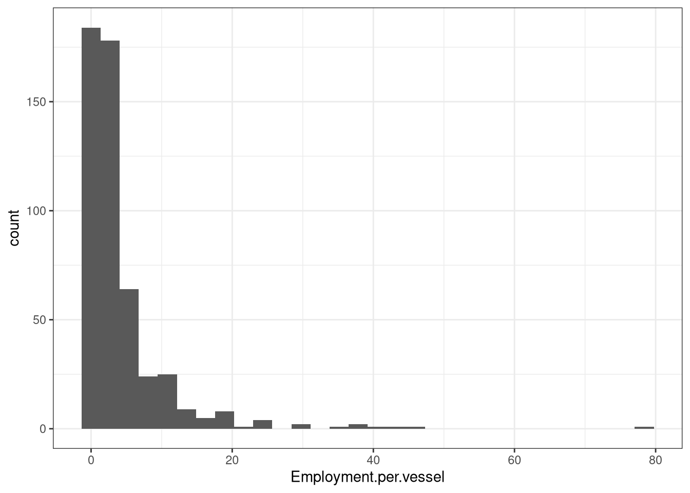

Figure 11: Employment per vessel

This is a potentially problematic metric, in retrospect, as it is really a metric of vessel size…

QUESTION: Should we retain it? How should we normalise it if we keep it?

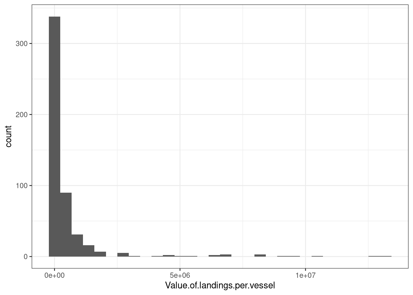
Figure 12: Value of landings

Hmmm. Similar problem.

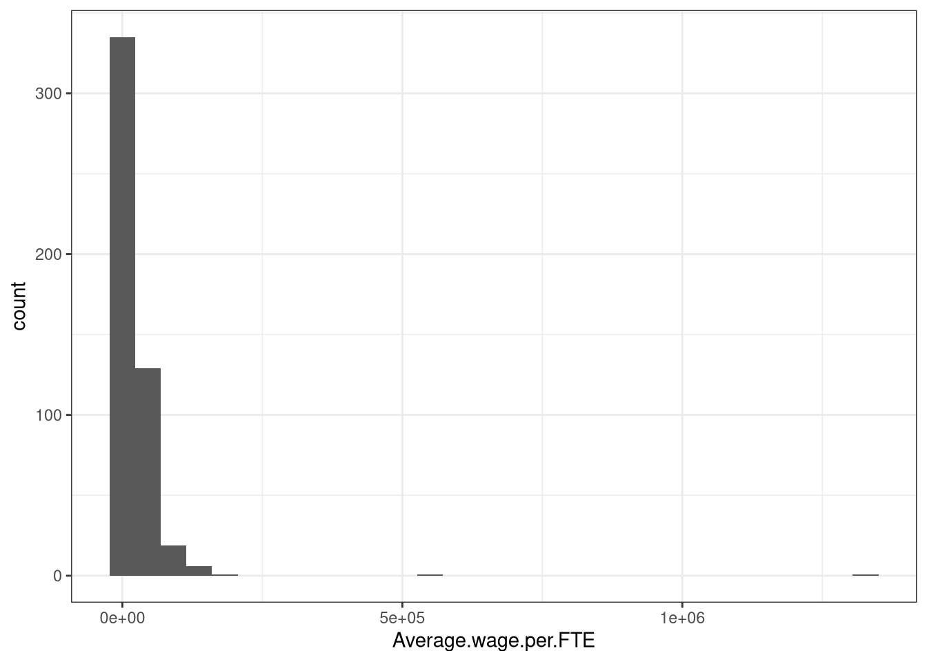
Figure 13: Average wage per FTE

Looks like a couple of outliers there that need to be polished up…

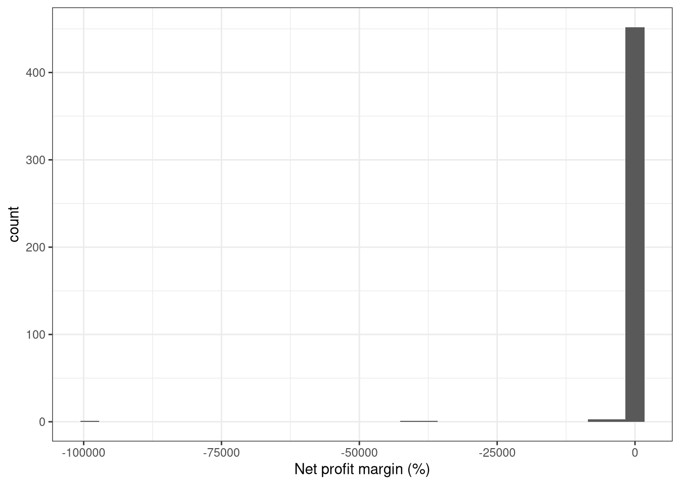
Figure 14: Net profit margin

Hmmm. A rather biased distribution. Lets crunch this figure down a bit…

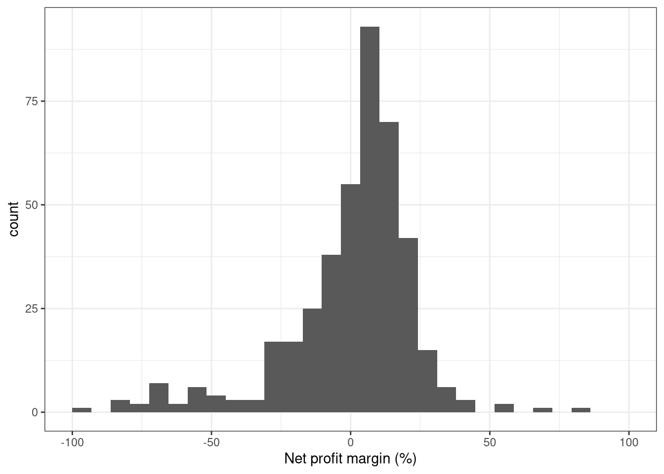
Figure 15: Net profit margin 2

Outliers aside, this is not a bad distribution.

QUESTION: Shall we rescale it to +/-50, and trim the rest…?

For the sake of this analysis, we have only based vulnerability on the Net Profit Margin, while we decide whether to include the rest..

Looking at the total vulnerability distribution.

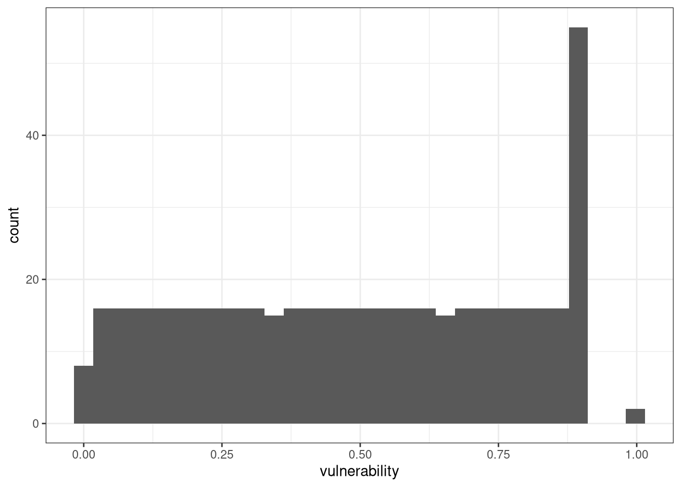
Figure 16: Vulnerability distribution

This doesn’t look so bad, but at the same time the outliers probably don’t help things, and should be fixed.

Checking the correlations with the metrics against vulnerability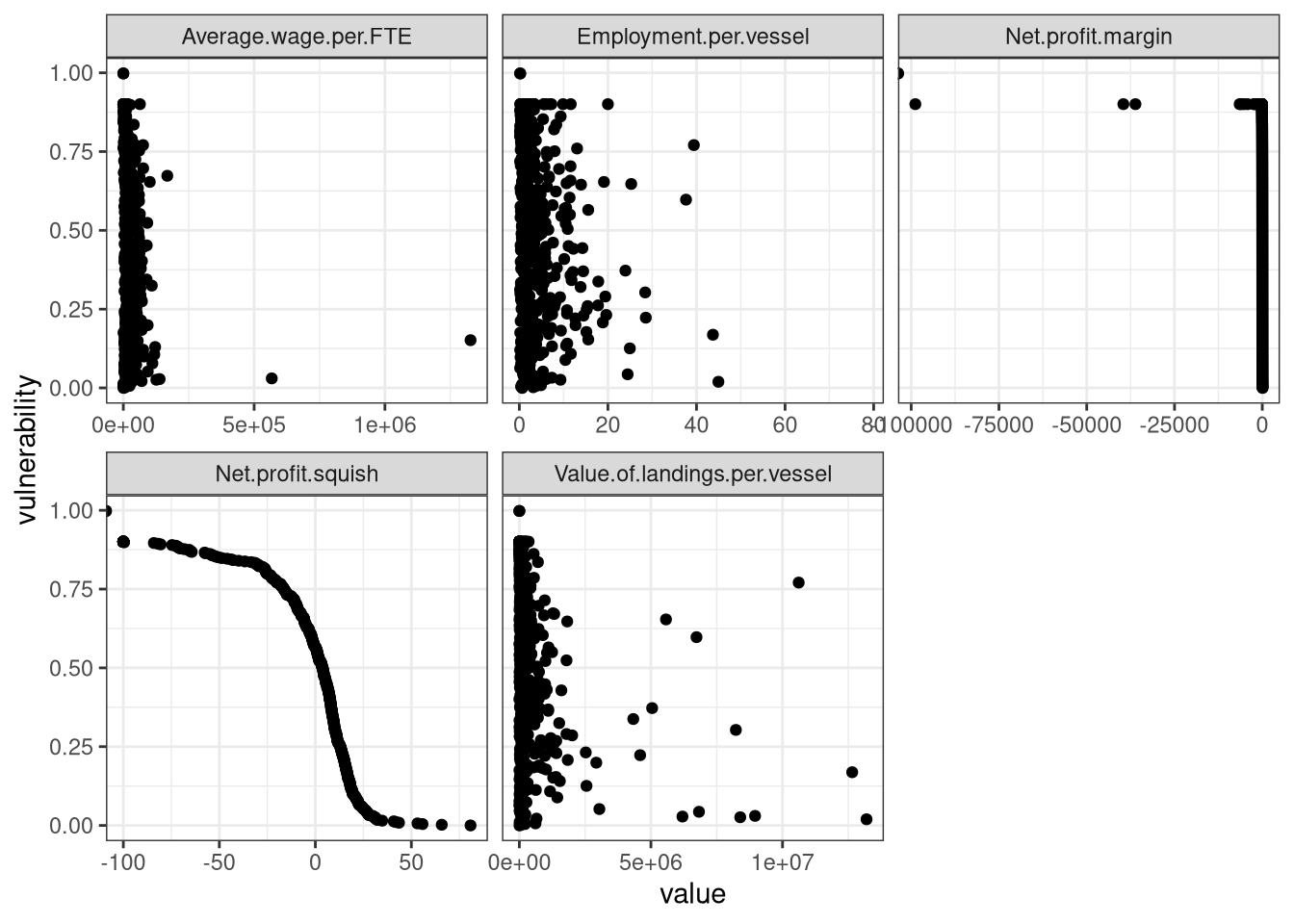

Figure 17: Correlation check

Which highlights the problems quite nicely… There is also some issues here with the directionality that we need to fix.

I think we probably need to rethink these metrics. Net profit margin is a very useful metric, but I’m not so sure about the others, particularly as they scale with vessel size, which I’m not sure we realy want…

4.3.4 Fleet risk

Note that the results here are a bit meaningless until we get the vulnerability under control, but the visualisations will be the same, so we can look at and discuss how we want to approach these.

Firstly, the top and bottom 10

Table 4: Top and bottom 10 fleets by risk

fs_name	country	area	gear	length	geo	total.val.landings	prop.missing	hazard	exposure	vulnerability	risk	country_name	country_2A
DNK A27 TM40XX	DNK	A27	TM	40XX		363359393.3	0.007	0.050	0.536	0.020	0.000	Denmark	DK
ITA A37 PGP0006	ITA	A37	PGP	0006		5721461.6	0.459	0.573	0.015	0.042	0.003	Italy	IT
PRT A27 DFN1012	PRT	A27	DFN	1012		356623.0	0.390	0.449	0.032	0.154	0.006	Portugal	PT
PRT A27 DTS0010	PRT	A27	DTS	0010		381875.0	0.275	0.491	0.141	0.025	0.008	Portugal	PT
ESP A37 DFN0612	ESP	A37	DFN	0612		630328.7	0.477	0.578	0.027	0.081	0.011	Spain	ES
ESP A37 DRB1218	ESP	A37	DRB	1218		167984.4	0.460	0.112	0.387	0.213	0.014	Spain	ES
PRT A27 PGP0010	PRT	A27	PGP	0010		9661098.0	0.206	0.323	0.176	0.230	0.017	Portugal	PT
ESP A27 PS2440	ESP	A27	PS	2440		34961229.8	0.174	0.146	0.333	0.258	0.020	Spain	ES
PRT A27 TBB0010	PRT	A27	TBB	0010		263508.0	0.439	0.367	0.149	0.249	0.022	Portugal	PT
ITA A37 PMP1218 °	ITA	A37	PMP	1218	°	449075.6	0.242	0.186	0.444	0.148	0.025	Italy	IT
IRL A27 TM0010 °	IRL	A27	TM	0010	°	114528.2	0.069	0.134	0.916	NA	NA	Ireland	IE
IRL A27 TM1218 °	IRL	A27	TM	1218	°	447382.0	0.607	0.221	0.692	NA	NA	Ireland	IE
IRL A27 TM2440	IRL	A27	TM	2440		31648490.3	0.067	0.087	0.429	NA	NA	Ireland	IE
IRL A27 TM40XX	IRL	A27	TM	40XX		125299317.0	0.067	0.067	0.613	NA	NA	Ireland	IE
POL A27 DTS40XX	POL	A27	DTS	40XX		6263477.9	0.012	0.266	0.896	NA	NA	Poland	PL
POL OFR TM40XX	POL	OFR	TM	40XX		53086199.0	0.635	0.826	0.769	NA	NA	Poland	PL
PRT A27 DTS1012	PRT	A27	DTS	1012		269941.0	0.392	0.591	0.117	NA	NA	Portugal	PT
PRT A27 PGP1824	PRT	A27	PGP	1824		167591.0	0.188	0.094	0.489	NA	NA	Portugal	PT
PRT A27 TBB1012 °	PRT	A27	TBB	1012	°	268783.0	0.611	0.243	0.313	NA	NA	Portugal	PT
PRT OFR HOK2440 IWE°	PRT	OFR	HOK	2440	IWE°	4408259.0	0.766	0.923	0.600	NA	NA	Portugal	PT

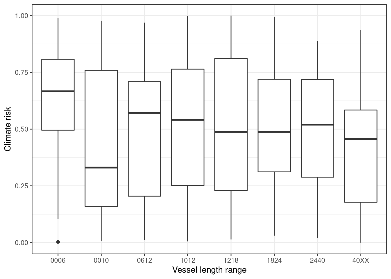
Now, viewing by vessel size

By country and fishing area.

QUESTION: I’m not quite sure how whether to retain the other fishing region fleets, or just keep it to the FAO27 and FAO37 areas - we don’t have very much biological information outside these regions.

QUESTION: I can also plot this as a map, based on the median value…

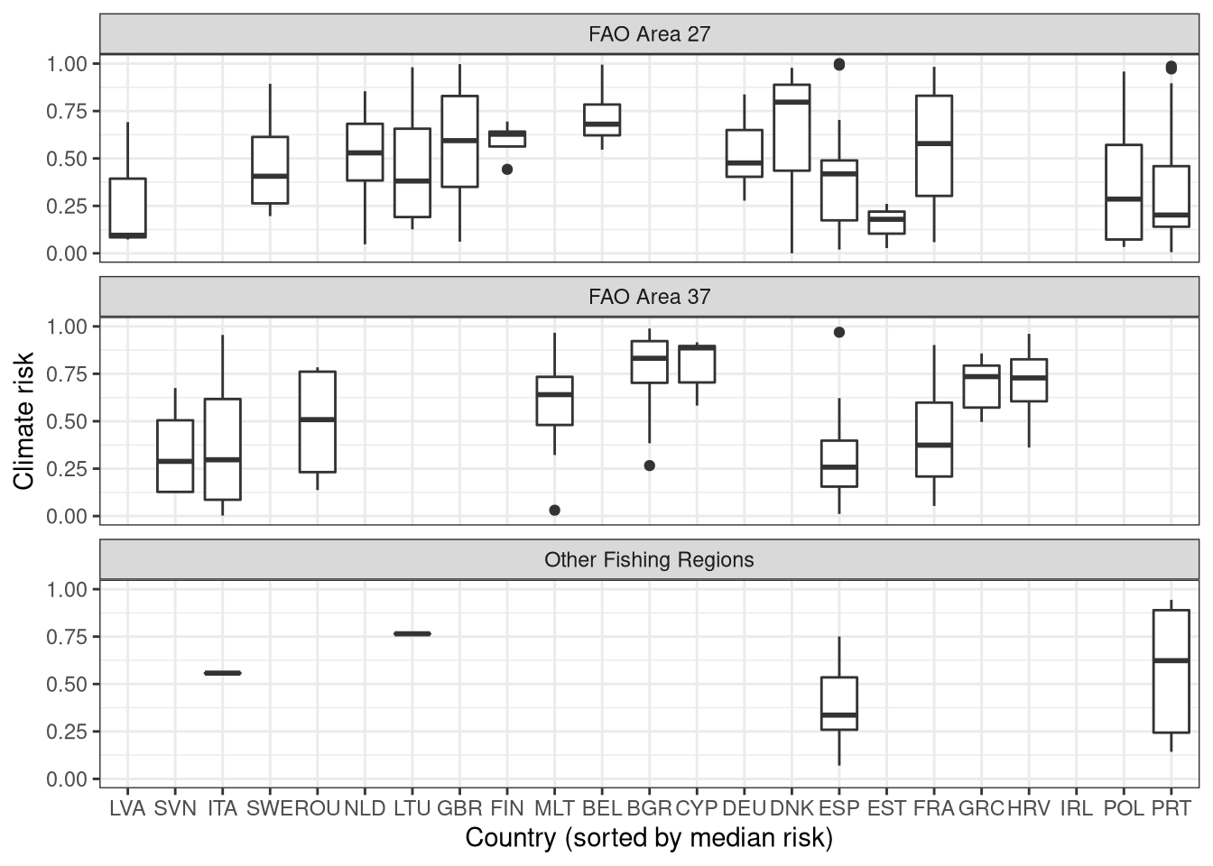
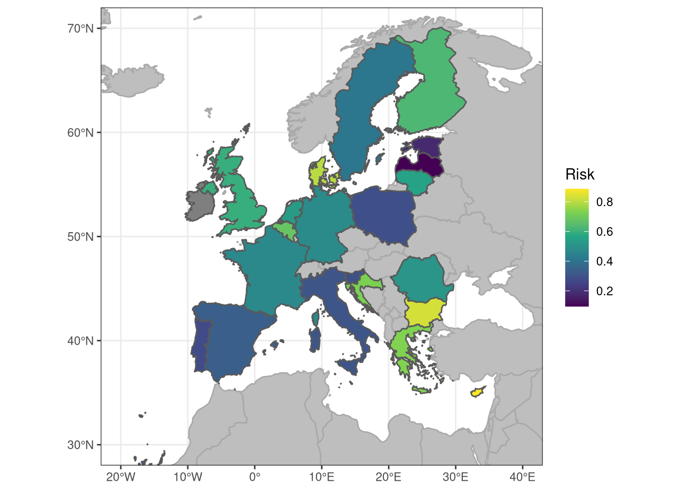
Figure 18: Fleetwise climate risk for the 23 EU coastal nations

TODO: Ireland needs to be investigated - it looks like it is missing some of the flet economic data => no vul => no risk.

TODO: I will separate France and Spain into Atlantic and Mediterranean fleets as well on this map

And by gear. Looks like quite some variability here.

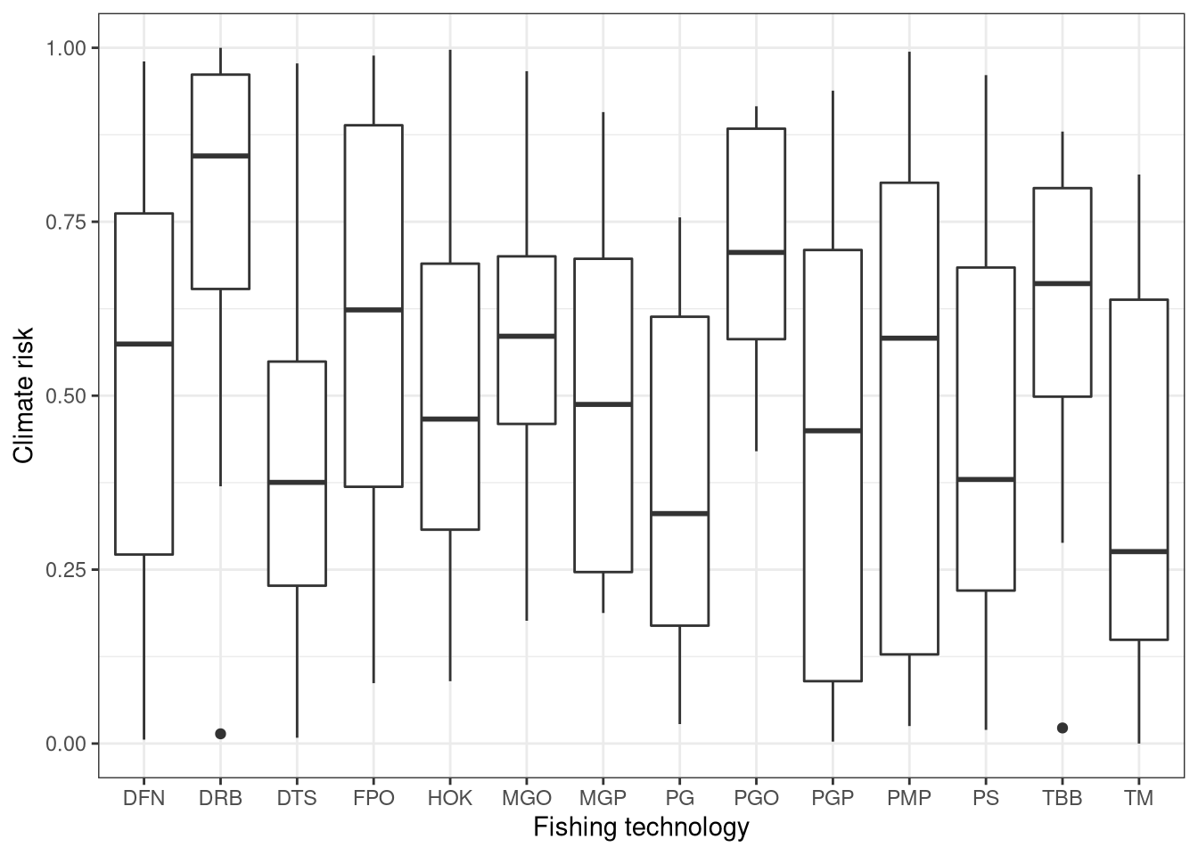
A table of gear types, sorted by median risk.

Code	Description	Risk
DRB	Dredgers	0.845
PGO	Vessels using other passive gears	0.706
TBB	Beam trawlers	0.661
FPO	Vessels using pots and/or traps	0.623
MGO	Vessel using other active gears	0.585
PMP	Vessels using active and passive gears	0.583
DFN	Drift and/or fixed netters	0.574
MGP	Vessels using polyvalent active gears only	0.487
HOK	Vessels using hooks	0.466
PGP	Vessels using polyvalent passive gears only	0.450
PS	Purse seiners	0.380
DTS	Demersal trawlers and/or demersal seiners	0.375
PG	Passive Gears	0.331
TM	Pelagic trawlers	0.276

4.4 Regional Metrics

4.4.1 Regional hazard

4.4.2 Regional exposure

Similar relationships between the catch dominance and catch diversity are seen at the regional levels as are seen for the fleets.

Check on the scaling and tendency

Plotting the exposure score geographically

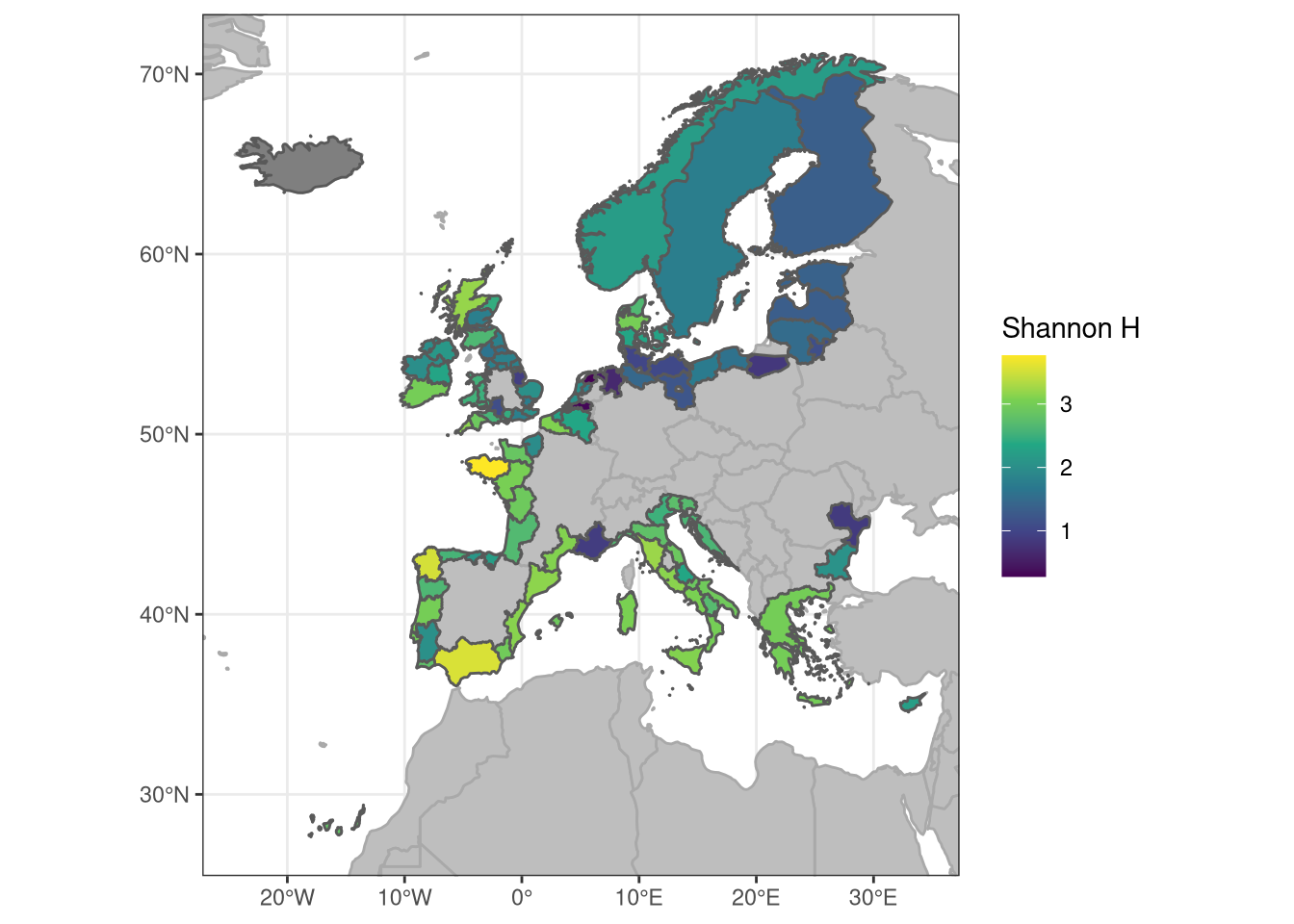
Note the clear north-south gradient here. Several countries are still missing from this analysis, as we don’t have data resolved by NUTS regions for them (e.g. Norway, Finland, parts of Sweden, SE Europe). We need to find a strategy how to deal with this.

4.4.3 Regional vulnerability

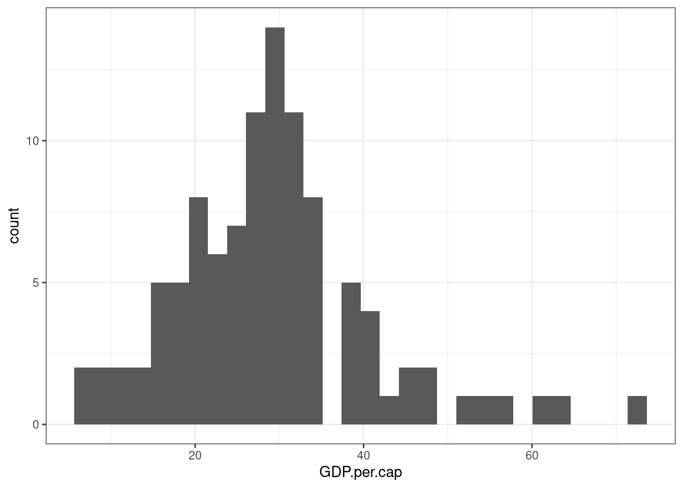
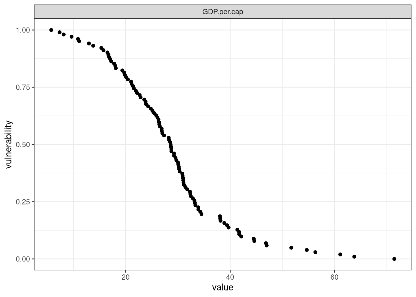
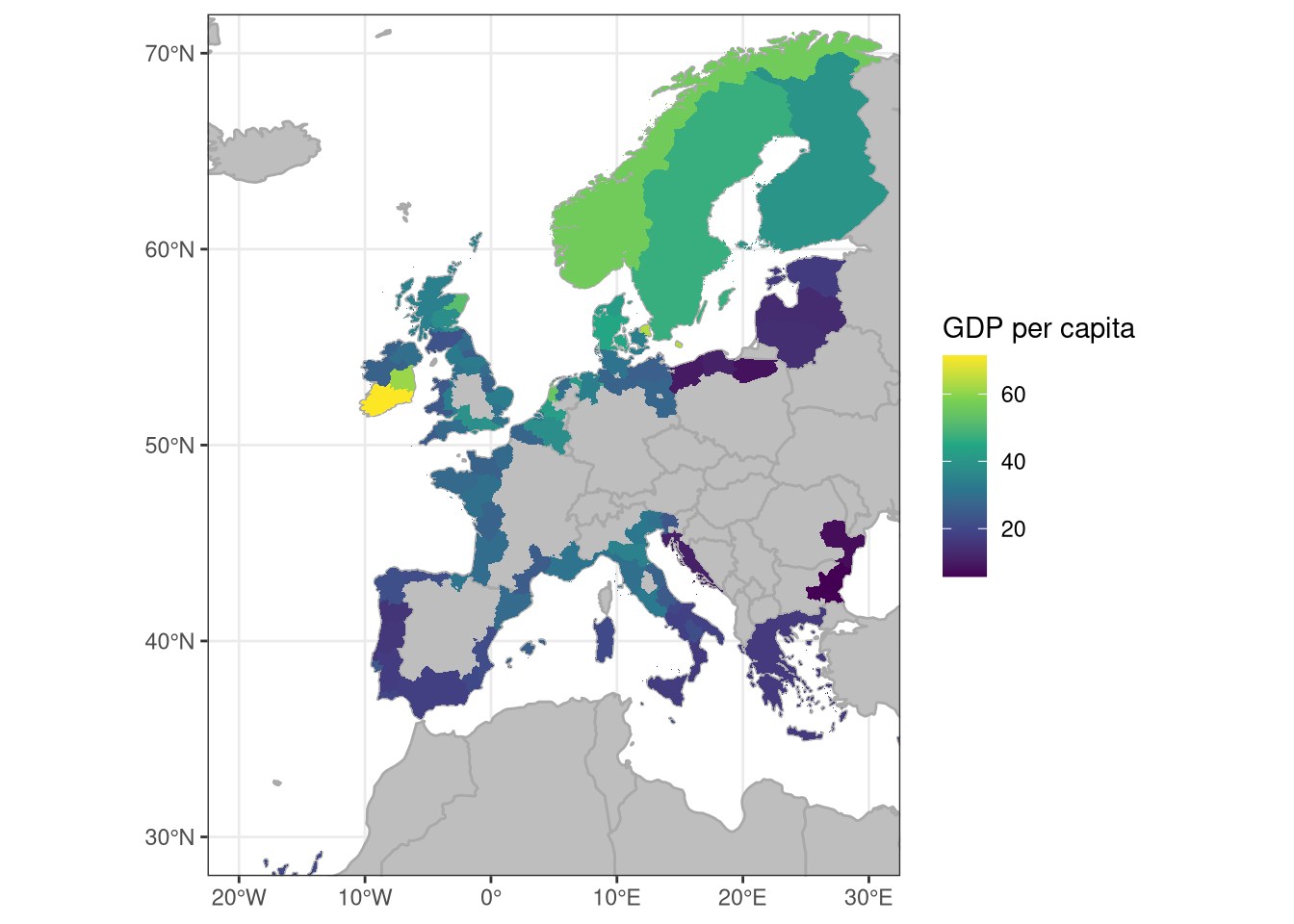
Currently this is only based on GDP per capita. Other metrics can be added. Plotting the distribution of values.

Checking the scaling and directionality

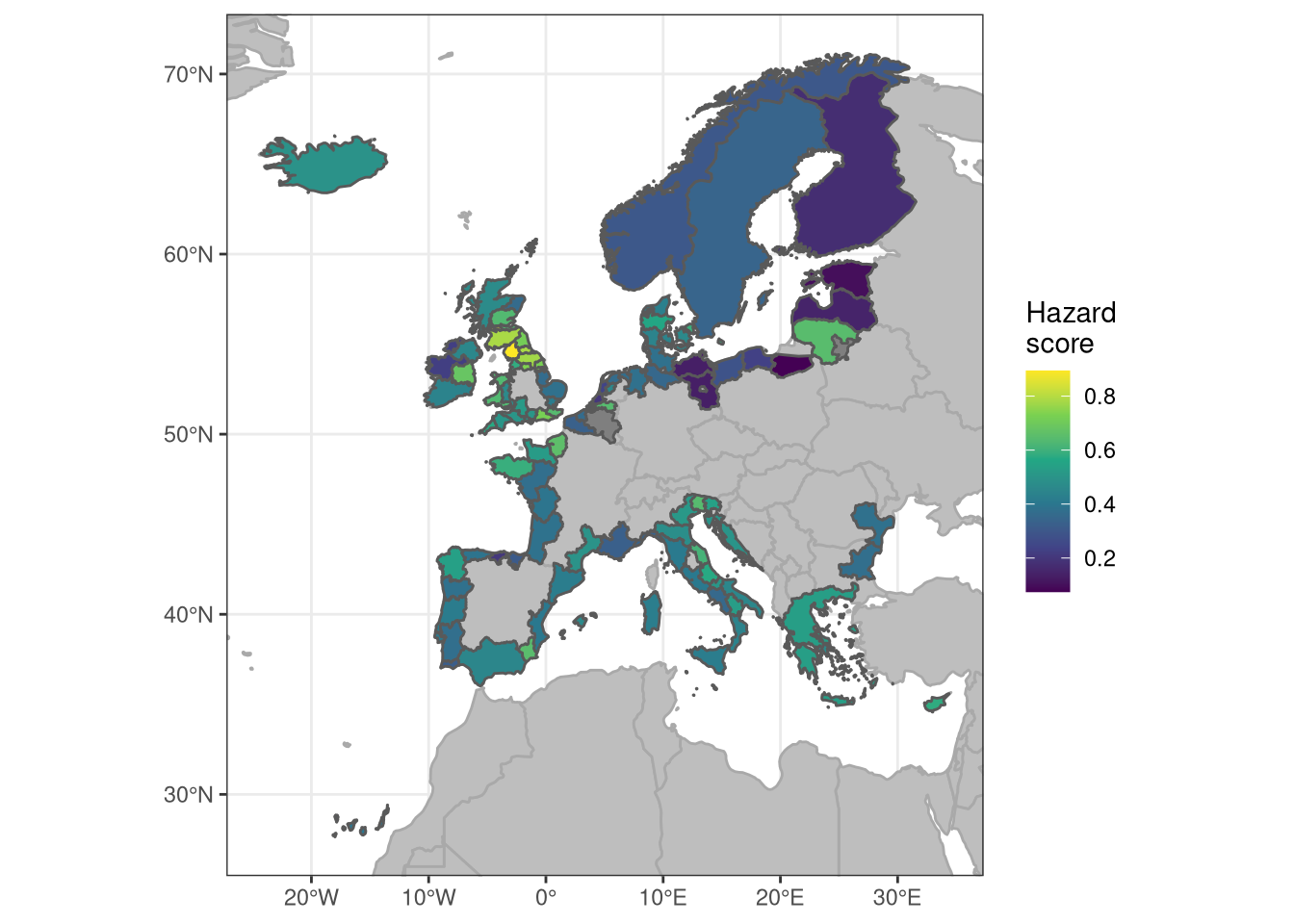
Distribution map.

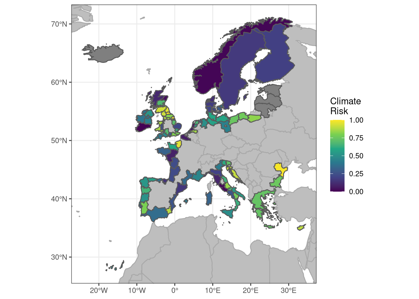
4.4.4 Regional risk

We calculate risk as the average of the hazard, exposure and vulnerability scores. This may need to be improved. The top and bottom ten regions by risk are then

Table 5: Top and bottom 10 regions by risk

region	hazard	exposure	vulnerability	risk	country
IE05	0.490	0.146	0.000	0.000	IE
NO	0.135	0.534	0.031	0.010	NO
ITI4	0.394	0.049	0.286	0.020	IT
UKM5	0.221	0.466	0.051	0.031	UK
NL32	0.115	0.612	0.041	0.041	NL
NL33	0.067	0.592	0.112	0.051	NL
DE50	0.096	0.621	0.071	0.061	DE
FRE1	0.173	0.087	0.561	0.071	FR
FRG0	0.279	0.126	0.418	0.082	FR
ITI1	0.413	0.019	0.429	0.092	IT
UKE1	0.942	0.718	0.510	0.969	UK
UKM8	0.990	0.903	0.296	0.980	UK
RO	0.298	0.961	0.990	0.990	RO
UKC1	0.971	0.835	0.653	1.000	UK
BE25	0.250	0.563	NA	NA	BE
EE00	0.010	0.854	NA	NA	EE
EL30	0.558	0.194	NA	NA	EL
IS	0.625	NA	NA	NA	IS
LT02	0.885	0.845	NA	NA	LT
LV00	0.038	0.864	NA	NA	LV

Putting it on a map

Putting it up as a boxplot

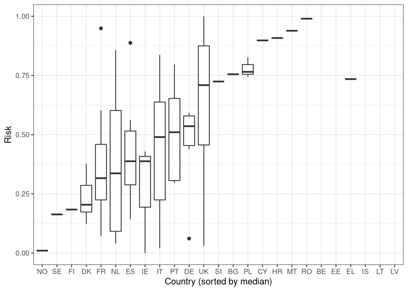
Interesting results. Lots of details there to discuss!