3 Methods
3.1 Analysis approach
The vulnerability analysis performed here follows the “new” risk-assessment framework developed by the IPCC in the Fifth Assessment Assessment report (AR5). This framework focuses on the climate-risk, which consists of the vulernability, exposure and climate hazard. In this work we consider two primary focii areas that are at risk from climate change - European fishing fleets and European regional communities.
TODO: Define fleets and communities (??)
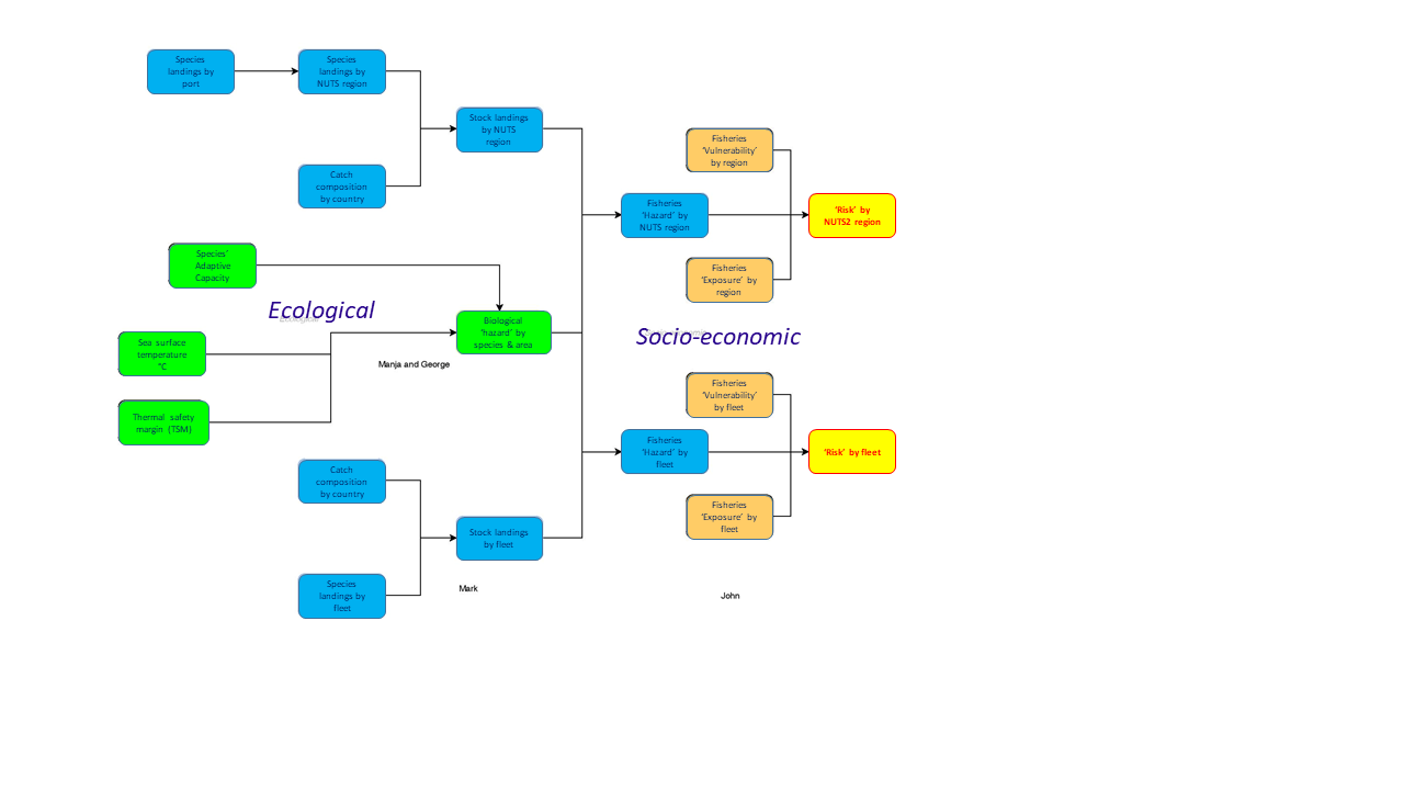
Both of these sectors are at risk from the impacts of climate change on the living marine resources upon which they depend. The biological impacts therefore form the base of this analysis (Figure xxx) and we consider two different mode of biological response. Firstly, species-specific harzards arise due to the inherent traits of the organism that can make it more, or less, sensitive to climate change. Secondly, the response also depends on the spatial context: a population of a given species that is close to its physiological upper thermal limit will be much more sensitive to warming than a population that is in the middle or colder part of its range. The combination of species-level information with the spatial context allows us to calculate the stock- (or population-) specific hazards that form the basis of this analysis.
The stock-specific hazards then propigate into the two main focii areas in different ways. In the case of the fleet analysis, this happens via the relative composition of the stocks that that each fleet fishes on, while in the case of the regional analysis it happens via the composition of the species that are landed in that region. These two different hazards are then combined with relevant vulnerability and exposure metrics to determine the overall climate risk in each focal area.
We focus primarily on “negative” effects of a changing climate resulting from warming temperatures. We do not consider the effect of other processes, such as ocean acdificatio, deoxygenation or other changes in the ocean system. We also consciously exclude the effect of cooling temperatures in some regions associated with climate change, which only impacts a minor fraction of the ocean. We also deliberately focus on “negative” of climate change to aid interpretation of the final results. Many climate vulnerability or risk analyses fail to adequately distinguish between positive and negative effects of climate change, and simply highlight elements of their study system that will change, without saying which direction. Such an approach can be difficult to interpret, and we therefore make a conscious decision to focus on “negative” impacts, so as to ease interpretation of the results.
3.2 Data sources
3.2.1 Fisheries data
TODO: Add details about preparation and polishing, temporal averaging etc.
- EUROSTAT Catch
- Covers 26 countries, including Iceland, Norway and Turkey
- Product: “Landings of fishery products - main data (fish_ld_main)”
- Resolved by country, species, weight and value
- Url: http://ec.europa.eu/eurostat/web/fisheries/data/database
- Product: Catches by fishing area (fish_ca_atl21, fish_ca_atl27, fish_ca_atl34, fish_ca_atl37)
- Catches by FAO area, country and species
- Url: http://ec.europa.eu/eurostat/web/fisheries/data/database
- EUMOFA Landings
- European Market Observatory for Fisheries and Aquaculture
- Provides monthly data on the value of landings broken down by species and port.
- Covers approximately 100 species in category groups
- 16 countries, including Norway
- Can be linked to NUTS 2 regions via Annex 8 correlation tables and with additional data provided by EUMOFA (Personal communication from Valentina Sannino, EUMOFA)
- Direct link: https://www.eumofa.eu/web/eumofa/bulk-download
- STECF Landings
- Provides the value of landings by fleet and species for 400 fleet segements
- 2018 Annual Economic report
- downloaded from the web portal https://stecf.jrc.ec.europa.eu/dd/fleet.
- “2018-07_STECF 18-07 -EU Fleet Landings FAO Gear levels_final” - landings by fleet segement, FAO area, species
- Only covers the 23 EU coastal states. No Norway or Iceland
3.2.2 Economic data
- EUROSTAT Economics
- Gross Domestic Product by NUTS3 region Product id: “nama_10r_2gdp”
- Population by NUTS3 region. Product id: “nama_10r_3popgdp”
- Unemployment rate by NUTS3 region. Product id:“lfst_r_lfu3rt”
- STECF Economics
- Provides economic characteristics of approximately 400 fleet segements
- 2018 Annual Economic report
- downloaded from the web portal https://stecf.jrc.ec.europa.eu/dd/fleet.
- “2018-07_STECF 18-07 - EU Fleet Economic and Transversal data_fs level_final” provides economic data
- Only covers the 23 EU coastal states. No Norway or Iceland
3.2.3 Biological data
- Pecuchet trait database
- Engelhardt trait database
- Aquamaps
3.2.4 Supplementary data
- FAO Area Polygons
- Polygons of the FAO fishing areas
- Direct link: http://www.fao.org/geonetwork/srv/en/main.home?uuid=ac02a460-da52-11dc-9d70-0017f293bd28
- Additional Link: http://www.fao.org/geonetwork/srv/en/main.home?uuid=ac02a460-da52-11dc-9d70-0017f293bd28
- Downloaded 17 July 2017
- FAO Species Codes
- Provides a systematic taxonomy covering around 11 000 (??) marine species.
- Direct link: http://www.fao.org/fishery/collection/asfis/en
- GCFM General Statistical Areas
- Url: http://www.fao.org/gfcm/data/maps/gsas
- Shapefiles: http://www.fao.org/fileadmin/user_upload/faoweb/GFCM/Maps/GSAs_simplified.zip
- Shapefiles contain a mapping between GSAs and FAO Subareas. Used to aggregate STECF fleet information in the mediterranean from GSAs to FAO Subareas.
- NUTS2 2016 Regions
- General information available here https://ec.europa.eu/eurostat/web/gisco/geodata/reference-data/administrative-units-statistical-units/nuts
- We used the NUTS 2016 1:10 million version shapefile, here: https://ec.europa.eu/eurostat/cache/GISCO/distribution/v2/nuts/download/ref-nuts-2016-10m.shp.zip
- EUMOFA correspondence keys
- Correspondence key linking FAO (ERS) species codes with EUMOFA’s “main commercial species” (MCS) codes downloaed from EUMOFA website
- Updated version of key linking harbor name and geographical location provided directly by EUMOFA
3.3 Biological Metrics
3.3.1 Preselection of Species
European fisheries cover an extremely broad range of biogeographic zones, ranging from the near-tropical waters of North Africa to the near-polar waters of the Barents Sea: distant water fleets expand this range even further to include essentially all of the world’s oceans. This results in an unmanagably large number of species that could be included in this analysis. We therefore first performed an initial screening to narrow this set of species down to a more manageable size. We employed the value of landings data provided by the “EUROSTAT catch” dataset to select species that cover 90% of landings by value, both at the European wide level and on a country-by-country basis. This analysis narrowed the 1200 species reported in this database down to 185 species groups. Entries that were not taxnomically resolved to either species or genus level were removed from the analysis, as it was deemed to be too difficult to extract representative biological information at such a coarse level.
This initial species list contained 24 entries that were only taxonomically resolved to the Genius level (“bucket categories”). For the purpose of defining traits and further analysis, exemplar species were chosen to represent this group. In some cases, it was necessary to use different exemplars for the North Atlantic (FAO 27) and Mediterranean regions (FAO 34) (see supplementary material). Furthermore, two species that are predominately freshwater, European perch (Perca fluviatilis FAO code FPE) and Pike-perch (Sander lucioperca FAO code FPP) were also removed from the database. Two further groups, Barnacles (Pollicipes pollicipes FAO code PCB) and Solen razor clams (Solen spp FAO code RAZ) were also removed, as it was not possible to find appropriate Aquamaps or identify suitable exemplars. Alternative (and misspelled) scientific names were also a problem in many cases. A list of corrections is also supplied in the Supplementary Material.
3.3.2 Species-specific metrics
TODO: * Response of an organism to climate change depends on its inherent characteristics (traits) * Traits are important short-hand for climate sensitivities and are widely used.
However, a key point that is often overlooked in many climate vulnerability analyses is that biological traits are often correlated. For example, small fish tend to have short life-spans, fast growth rates and sit on relatively low trophic levels, while large fish live longer, grow slower and are near the topic of the foodweb. Disregarding these correlations between traits can therefore bias the analysis.
Previous work (Pecuchet et al. 2017) has shown that fish communities in European seas can be readily decomposed into three life-history strategies (LHS), based on their traits. Maximum length, lifespan and trophic level were highly correlated with each other and formed the primary axis discriminating the “opportunistic” LHS identified in this paper. This LHS was also shown to be associated with seasonal and variable environments, and there implies robustness to change and variability. Following from these conclusions, we employed one metric of this axis, the Lifespan, as an indicator of sensitivity to climate change, with shorter lifespans being associated with reduced sensitivity.
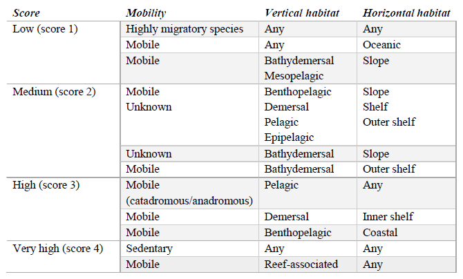
TODO: * Habitat specificity traits. Three traits were combined and scored (see table) + a low score infers low habitat specificity or good adaptive capacity +a high habitat specificity score indicates a species with low adaptive capacity.
We used the trait database developed by Pecuchet et al 2017 (TODO: reference to Panagea dataset) and Engelhardt et al 2011 as the primary sources of trait information for the species considered in this work. Traits for species that were not covered by these two databases were filled based on literature searches (e.g. shellfish), primarily from Fishbase and Sealifebase.
3.3.3 Species-specific metrics
We use habitat maps generated by the website http://www.aquamaps.org to form the basis for estimating thermal safety margins and for placing species in a spatial context. This website produces standardized distribution maps of over 25 000 species, based on empirically-derived species distribution models. We downloaded “native distribution maps” from the Aquamaps website for all of the species above, except for Purple Whelk (Rapana venosa FAO code RPW). This invasive species, originally from waters around Japan, Korea and China, now supports a large fishery in the Black Sea: for this species, the “Suitable Habitat map” was used rather than the “native distribution map”. In many cases, Aquamaps contains many multiple distribution maps for the same species, and the map was therefore chosen based on the internal map quality ranking system (“Expert reviewed” > “Team reviewed” > “Computer generated”).
We illustrate the use of Aquamaps to generate data using Atlantic cod (Gadus morhua) as an example.
The Aquamap for this species looks like so:
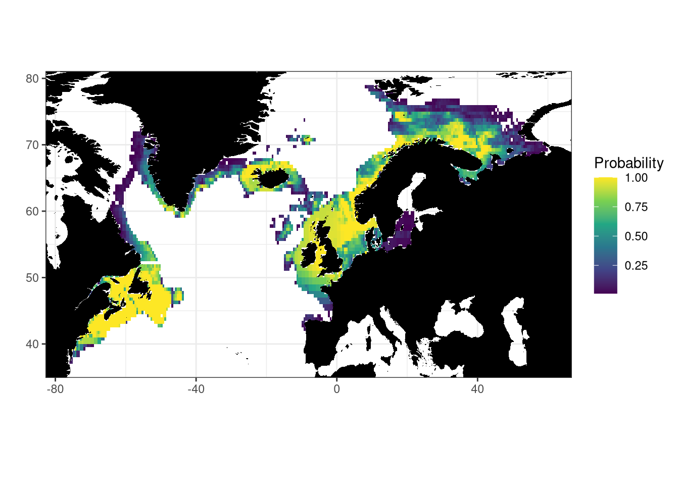
Figure 1: Aquamap native distribution map for Atlantic cod
The thermal envelope fitted for this species by Aquamaps looks like so.
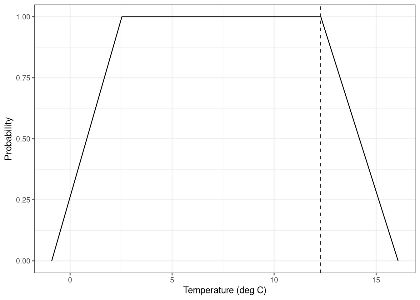
Figure 2: Thermal preference curve for Atlantic cod as fitted by Aquamaps. The dashed vertical line indicates the upper-thermal limit applied here.
Aquamaps chooses either SST or SBT, depending on the characteristics of the species.
It is clear that are high temperatures, the probability of a point in space being suitable habitat falls off to zero. In Aquamaps terminology, the point where this starts is the 90th percentile of the distribution, and we use this as the basis for defining the thermal safety margin, TSM, as follows.
\[TSM_i=T_{90^{th}}-T_{i}\]
where \(TSM_i\) is the thermal safety margin of pixel i, \(T_{90^{th}}\) is the 90th percentile and \(T_i\) is the temperature at a given pixel.
TODO: Lots of references to the TSM concept
Aquamaps provides the environmental data that underlies its models. We use this data for all analyses to ensure consistency between the thermal envelope parameters and the spatial distribution of temperature used to calculate TSM. We use the habitat distribution from Aquamaps to filter this environmental data to regions where the species of interest is expected to occur. For Atlantic cod, this looks like so:
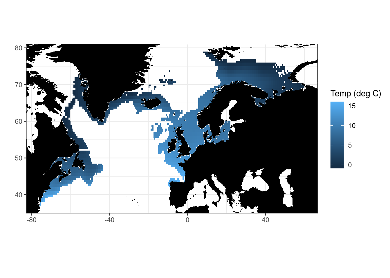
Figure 3: Aquamaps temperature for Atlantic cod
Combining the temperature with the thermal threshold allows us to calculate, and map, the thermal safety margin (TSM) as a function of space
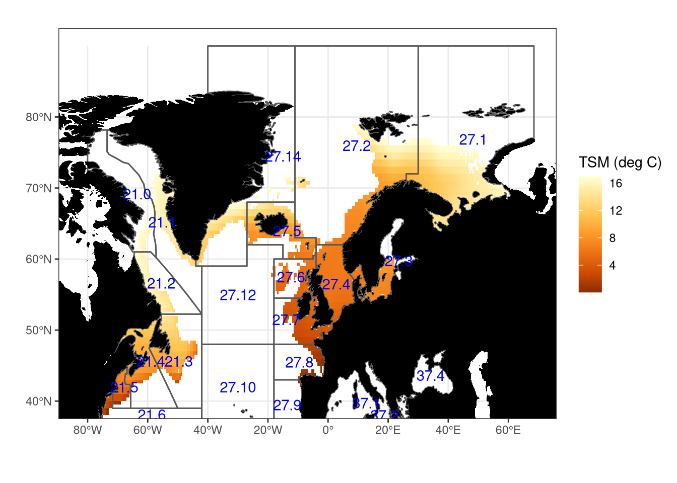
Figure 4: Aquamaps TSM (deg C) for Atlantic cod
In this case, we have also overlayed the FAO regions and labels. Focusing on a particular FAO region (e.g. 27.4), we can examine the statistical distributon of the TSM in the pixels that are deemed to be suitable habitat:
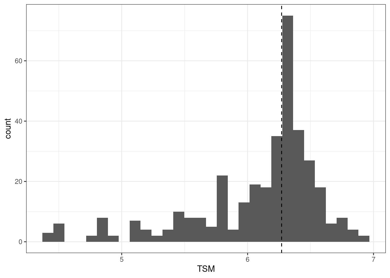
Figure 5: Distribution of TSM values for FAO region 27.4 The dashed vertical line indicates the median value.
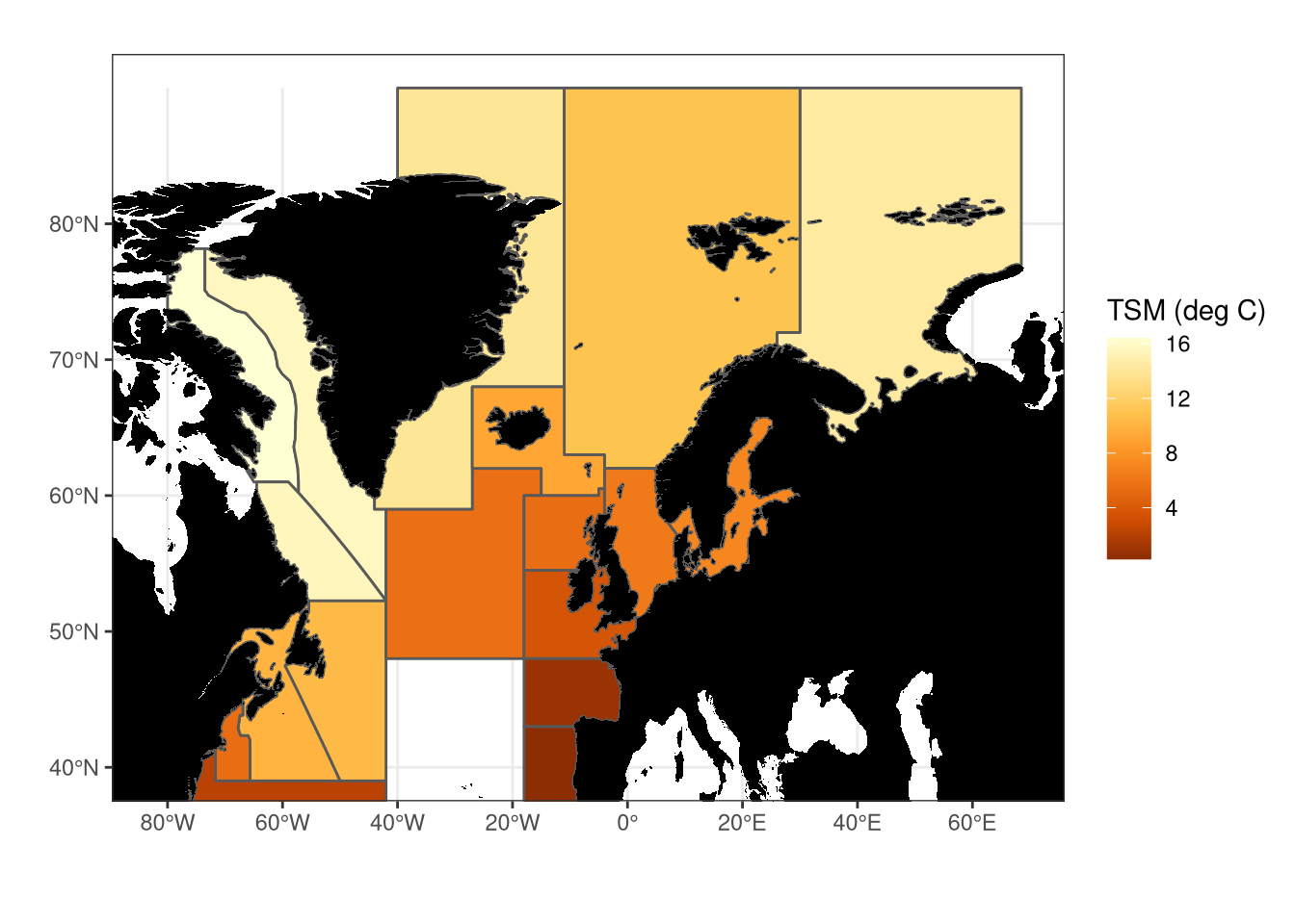
The median TSM for this species and area is used as a stock-specific metric of sensitivty to climate change. Stocks with low TSMs are viewed as being senstive, while those with high TSMs are viewed as being insensitive.
Applying this approach across all areas allows us to define a stock-specific TSM:
3.3.4 Combining metrics
We normalise all metrics on to a scale from 0-1 based on their relative ranks. We then produced a combined biological hazard metric for each stock as follows:
\[ H_{st}= 0.25LS_{sp} + 0.25 HSS_{sp} + 0.5 * TSM_{st} \] where \(H_{st}\) is the stock-specific hazard, \(LS_{sp}\) is the lifespan of the species, \(HSS_{sp}\) is the habitat-specificity score of the species and \(TSM_{st}\) is the stock-specific thermal-safety margin.
3.4 Fishing Fleet Metrics
According to the EU Data Collection Regulation (DCR), a fleet segment is defined by the gear code and the vessel length category
- FISHING_TECHNIQUE=gear codes -see codes below
- VESSEL_LENGTH=vessel length class -see codes below.
It defines the minimum and maximum vessel length of fleet segment.The segmentation to level 2 is defined in Appendix III of the Commission Regulation 1639/2001, to level 3 in Appendix VIII and to level 4 in Appendix X.
3.4.1 Fishing Fleet Hazard
TODO: * STECF provides the catches of each species from each FAO subarea (ie. for each stock) for each fleet segment * We weight the biological hazard score for each stock by the proportion of the value of landings coming from that stock for each fleet ie
\[ H_{fs} = \frac{\sum_{st}{V_{st,fs}H_{st}}}{\sum_{st}{V_{st,fs}}}\] where \(H_{fs}\) is the hazard of fleet segment \(fs\), \(V_{st,fs}\) is the value of landings from each stock for each fleet segment, and \(H_{st}\) is the hazard of stock \(st\).
3.4.2 Fishing Fleet Exposure
Fleet segments are more likely to be sensitive to climate change if they are highly dependent on a climate-vulnerable natural resource. Many authors have assumed that fleets, ports or fishing communities have higher resilience if they catch a wide range of fish species, rather than concentrating on a specific resource. In order to calculate such indices for the EU fishing fleets we made use of the catch statistics provided by the EU Scientific, Technical and Economic Committee for Fisheries (STECF). This yielded complete data for 423 fleet segments, as defined under the EU Data Collection Framework (DCF) and used throughout in the Annual Economic Report (AER). A fleet segment is the combination of a particular fishing technique category and a vessel length category.Landings data for the base year of 2016 were aggregated to the fleet-segment (FS) level. Following this, two indices were calculated, “Shannon diversity of fisheries landings”and “Simpson’s dominance of fisheries landings”.
The Shannon statistic (\(ShannonH_{fs}\)) is one of the most commonly used diversity indices in ecology. The formula for calculating the index for each fleet segment is
\[ ShannonH_{fs} = - \sum_{sp}{p_{sp,fs} \ln{p_{sp,fs}}}\]
where \(p_{sp,fs}\) is the proportion of landings of species \(sp\) in fleet segment \(fs\). \(p_{sp,fs}\) is calculated from the species and fleet segement resolved landings \(L_{sp,fs}\) as \(p_{sp,fs}=\frac{L_{sp,fs}}{L_{fs}}\), where \(L_{fs}=\sum_{sp}{L_{sp,fs}}\) is the total landings of that fleet segment.
Simpson’s dominance index (D) is another widely used statistic which, as the title implies, emphasizes the relative abundance of the commonest species in the sample, i.e. it measures the degree of dominance by a few key species. As D increases, dominance increases and therefore evenness and diversity decreases. The equation and calculation are as follows:
\[D_{fs} = \sum_{sp}{\frac{L_{sp,fs}(L_{sp,fs}-1)}{L_{fs}(L_{fs}-1)}}\]
Note that, in the present analysis, high diversity (\(ShannonH_{fs}’\)) of landings at the fleet segment level is thought to characterize fishing fleets that are less sensitive to climate change whereas fleet segments that exhibit higher dominance (\(D_{fs}\)) are thought to be more sensitive and hence these two indices have been scaled accordingly.
A composite index of fleet segement exposure \(FE\) was calculated as an unweighted average of the two indices described above. Resulting values were normalized and scaled to range from 0 to 1, with higher values reflecting greater sensitivity.
3.4.3 Fishing Fleet Vulnerability
We used four metrics of fishing fleet vulnerability
- Employment per vessel =
Full-time equivalent (harmonised)/Total number of vessels - Value of landings per vesssel =
Value of landings/Total number of vessels - Average wage per FTE =
Wages and salaries of crew/Full-time equivalent (harmonised) - Net profit margin, which was calculated as described in the 2018 Annual Economic report: briefly, this corresponds to Net profit margin =
These metrics were calculated for all years in which the fleet was active, and then averaged over the period 2011-2015. A combined vulnerability score was produced by rescaling all four metrics to have a range from 0 to 1, and averaging the result.
3.4.4 Fishing Fleet Risk
- Combination
- Visualisations
3.5 Regional Metrics
3.5.1 Regional units
TODO: Desirable to have a higher spatial resolution than national level.
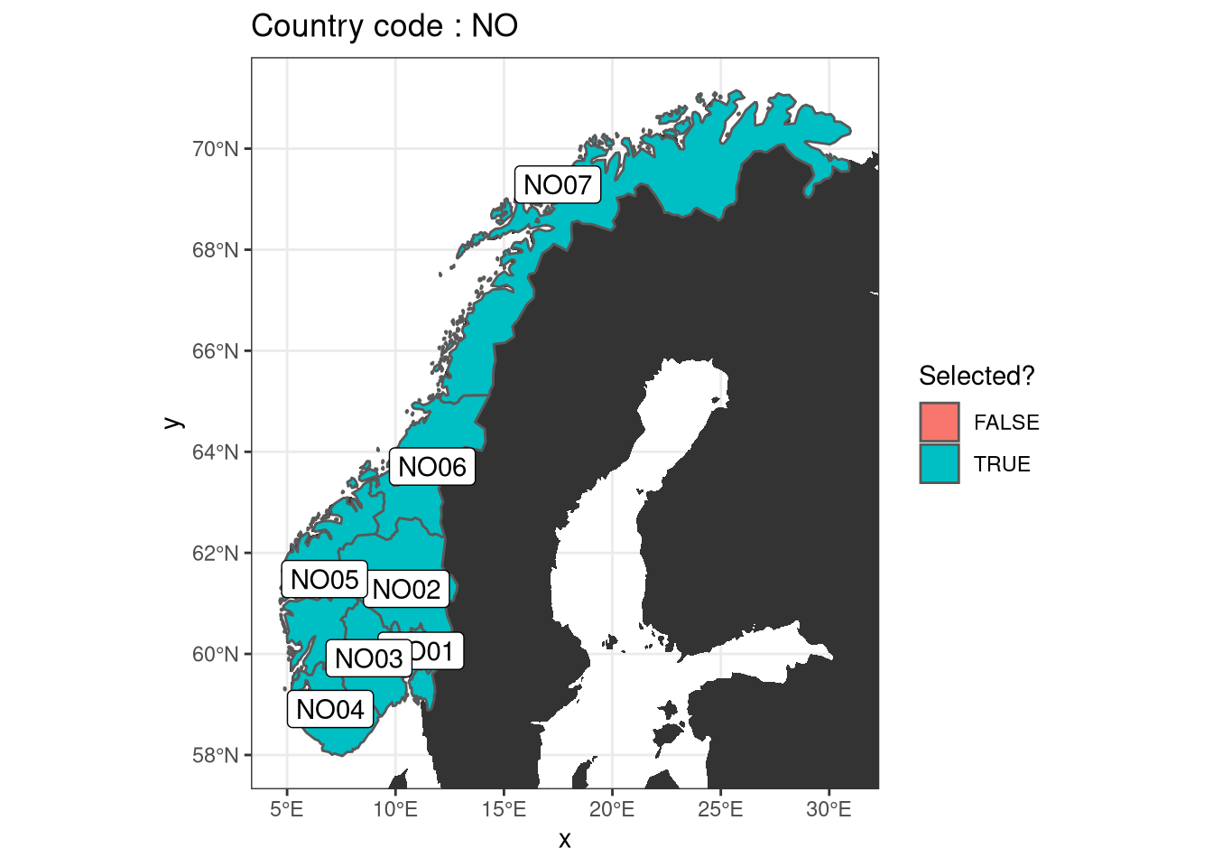
The EU Market Obsevatory for Fisheries and Aquaculture (EUMOFA) provides monthly “First-sale” records on a harbour-by-harbour basis for 16 European countries. We take advantage of this high spatial resolution to examine the climate hazard on a sub-national level, focusing on the NUTS2 regional units where possible. We first excluded Norwegian and Swedish from this analysis, as it was not on the same harbour-level resolution as for the other countries. We merged the EUMOFA first-sales data with geographical metadata (the longitude and latitude of each harbour) provided by EUMOFA, and used this spatial context to associate the harbour with the corresponding NUTS2 region.
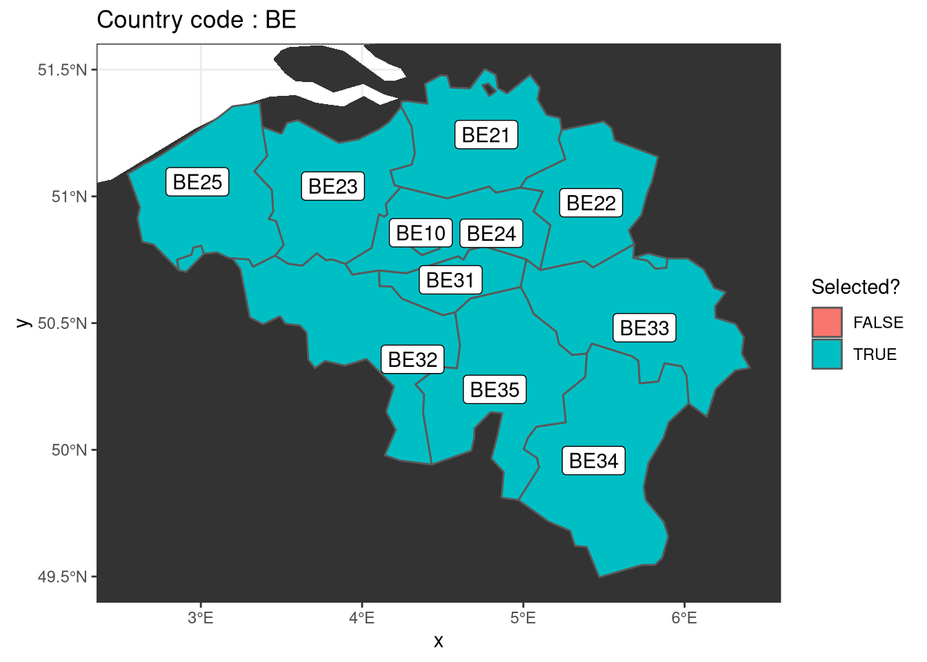
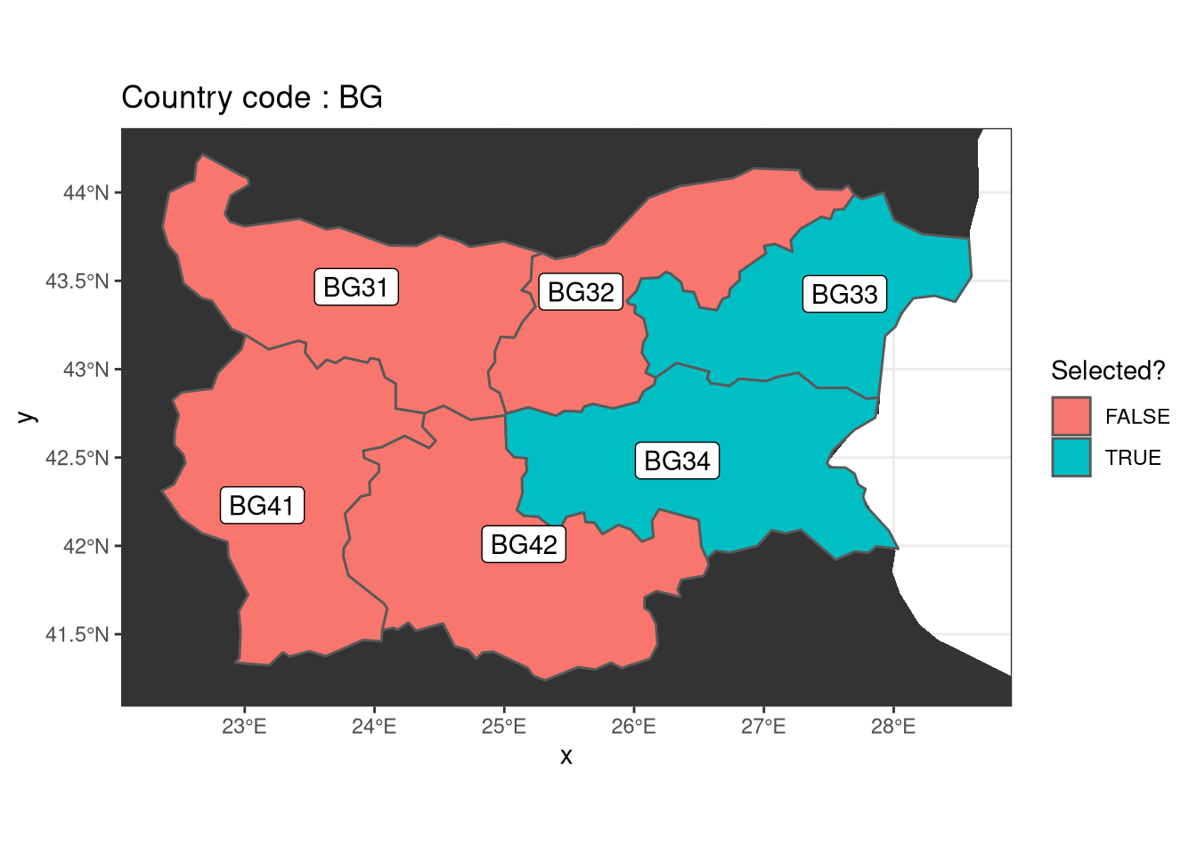
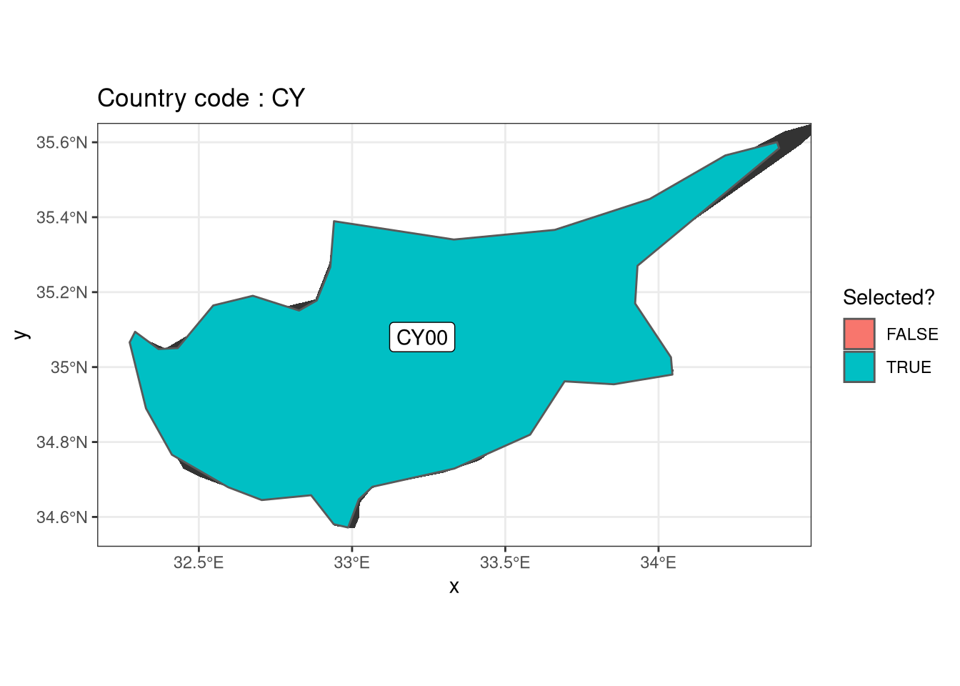
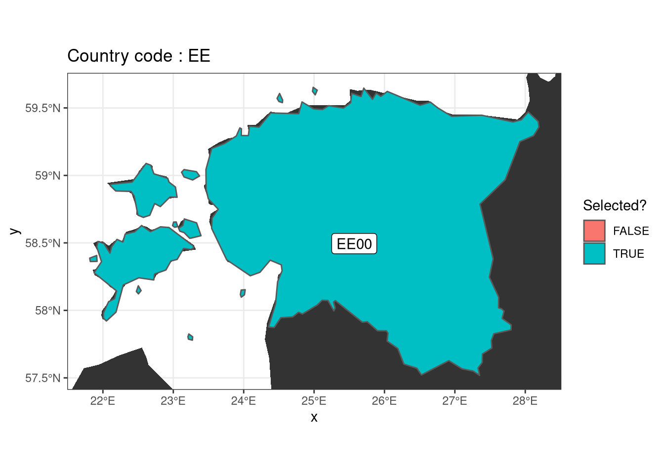
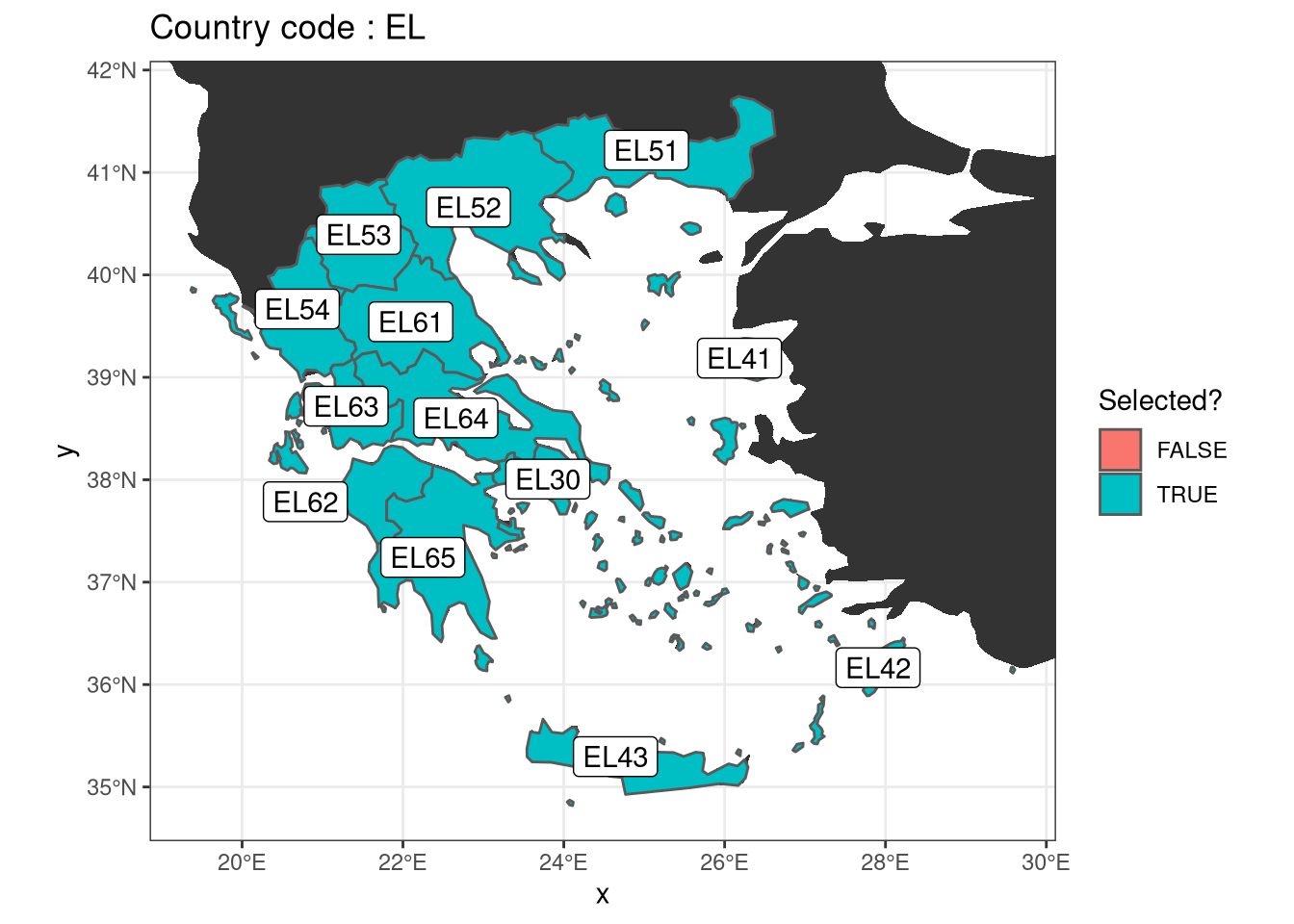
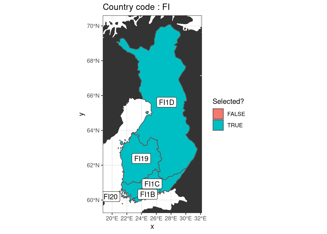
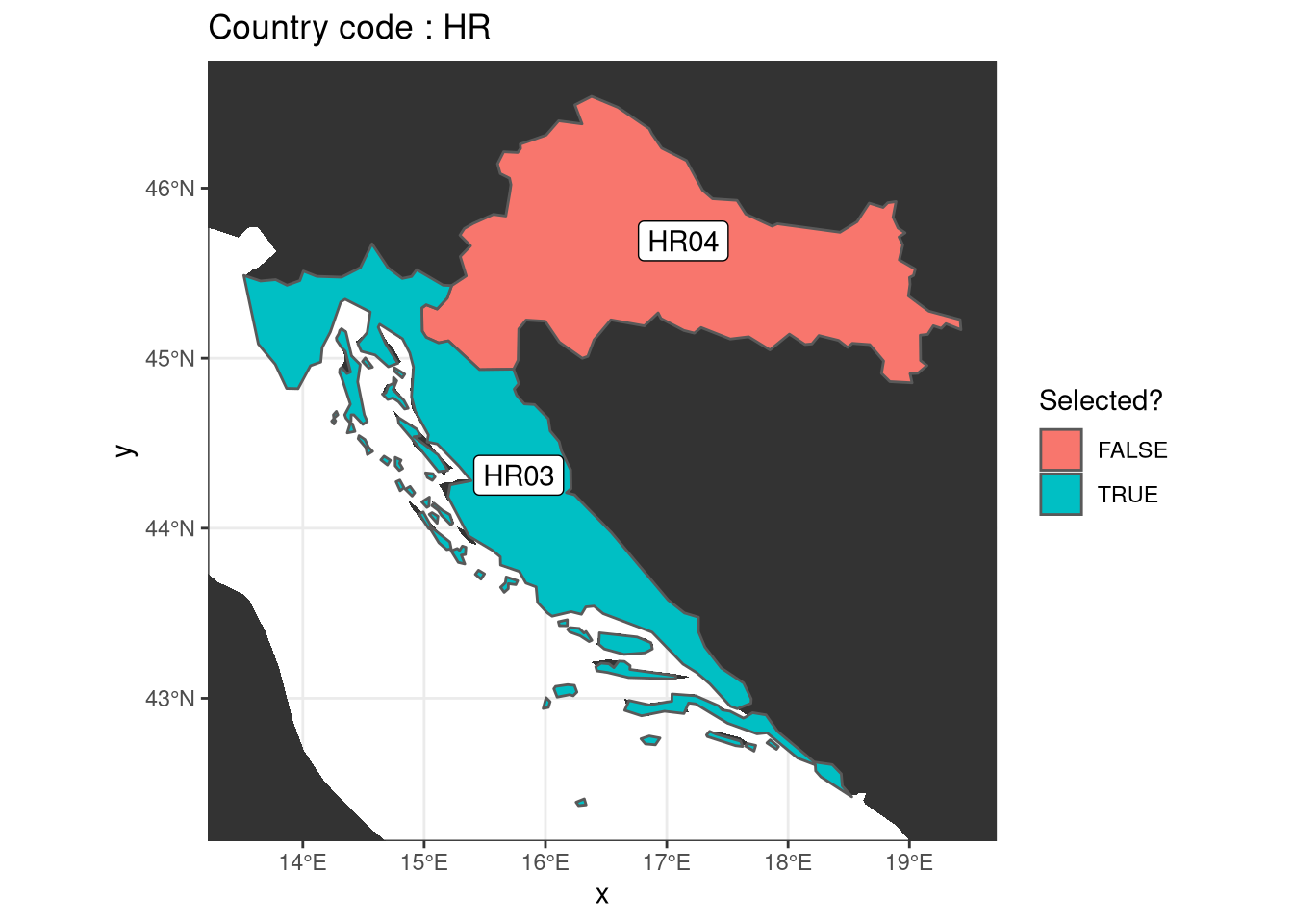
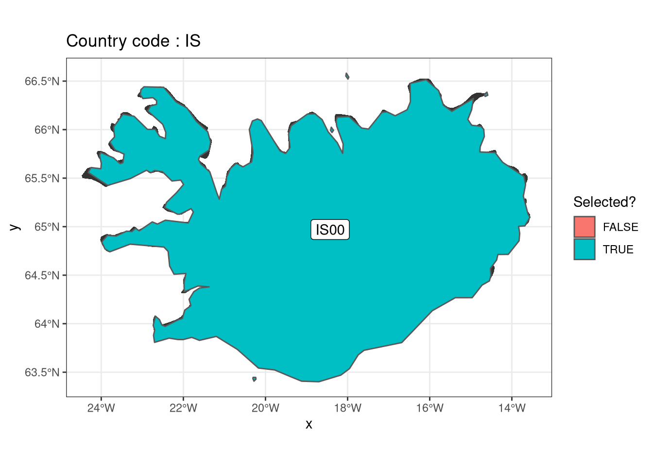
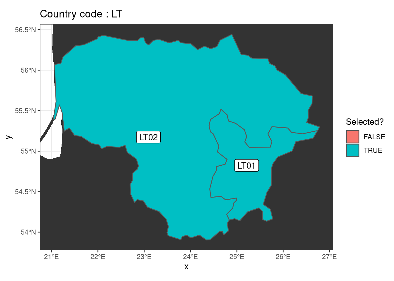
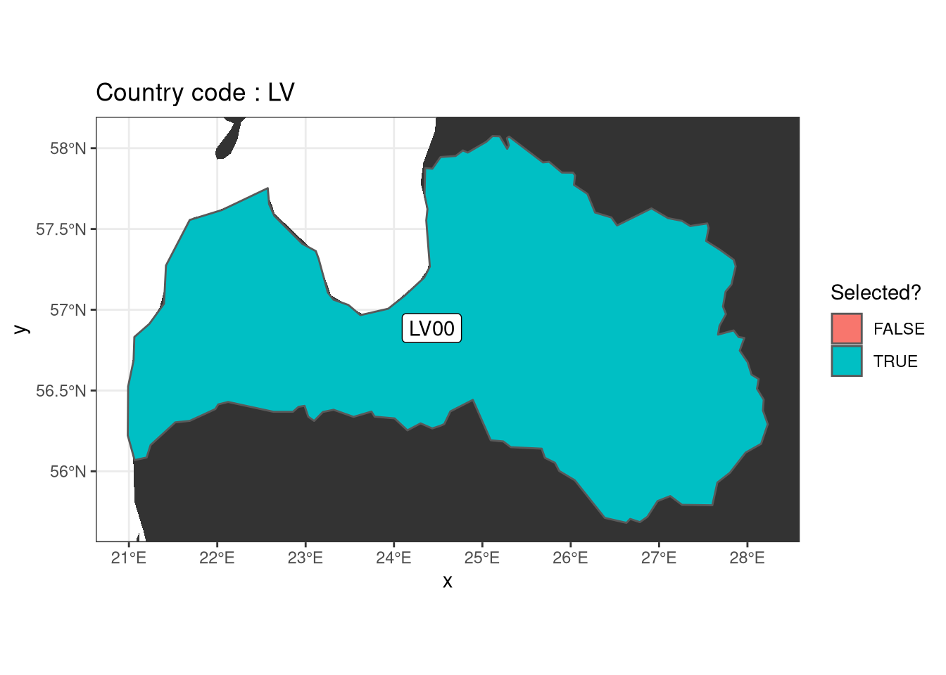
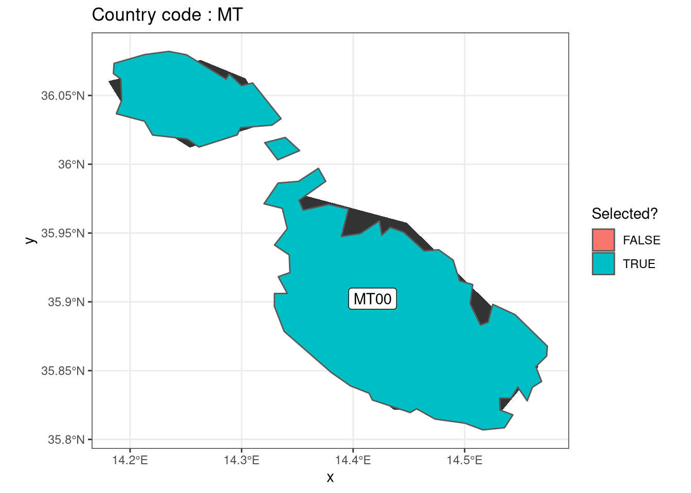
For countries not covered by EUMOFA, we generated a comparable database of landings based on the “EUROSTAT landings” dataset. We first aggregated the species resolution in EUROSTAT data from FAO species codes to the “Main commercial species” (MCS) groupings used by EUMOFA, based on correlation keys provided by EUMOFA, to ensure comparability between these data sets. We then associated these landings with the coastal NUTS2 regions in each country. In some cases (e.g. Iceland, Malta, Cyprus) there was only one NUTS2 region: however in other cases (notably Bulgaria) we generated new “regions” based on the union of multiple coastal NUTS2 regions. The new NUTS2 regions selected in each of these cases can be seen below:
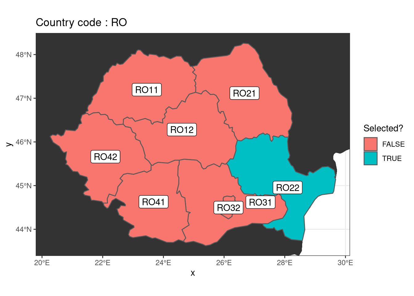
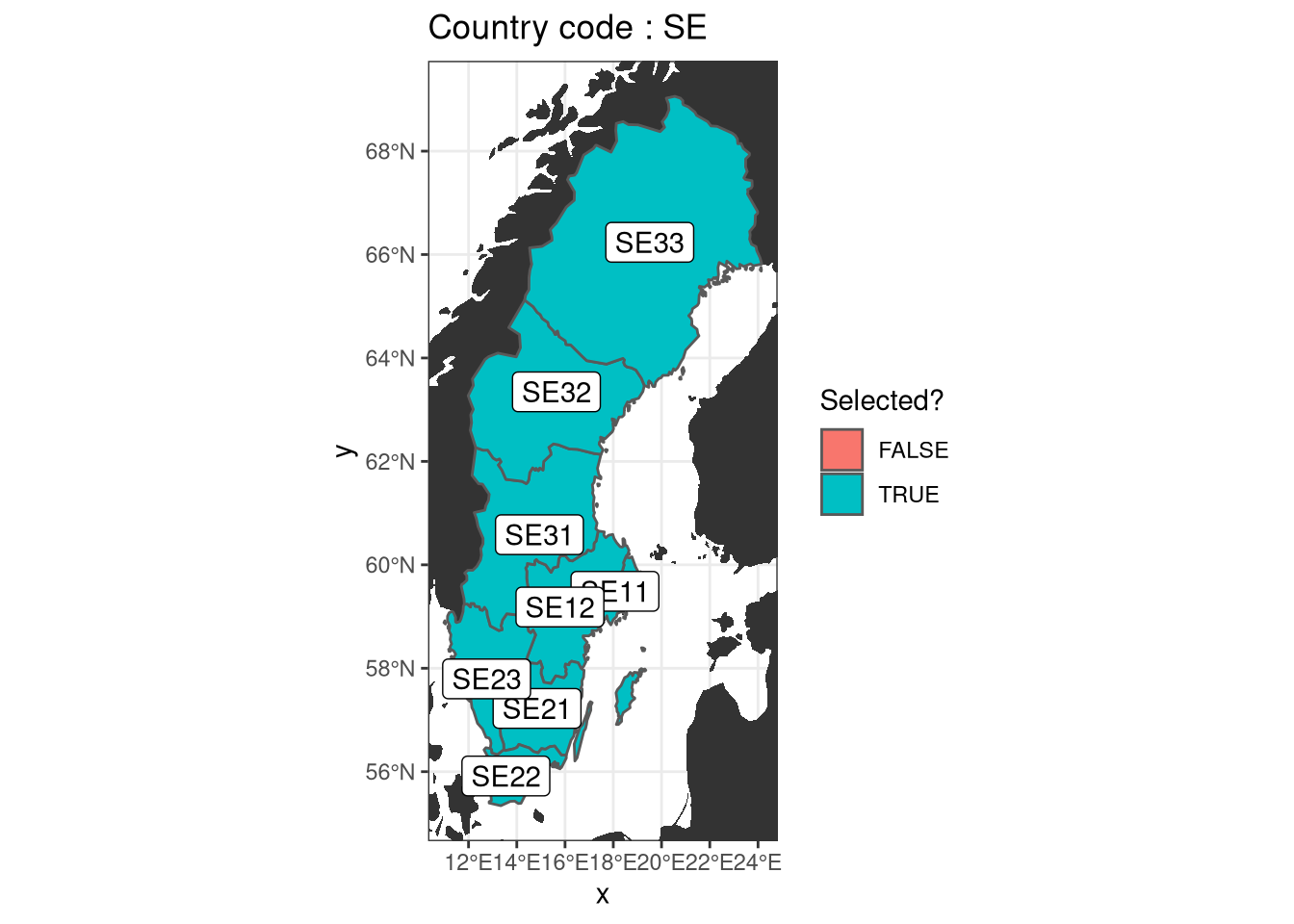
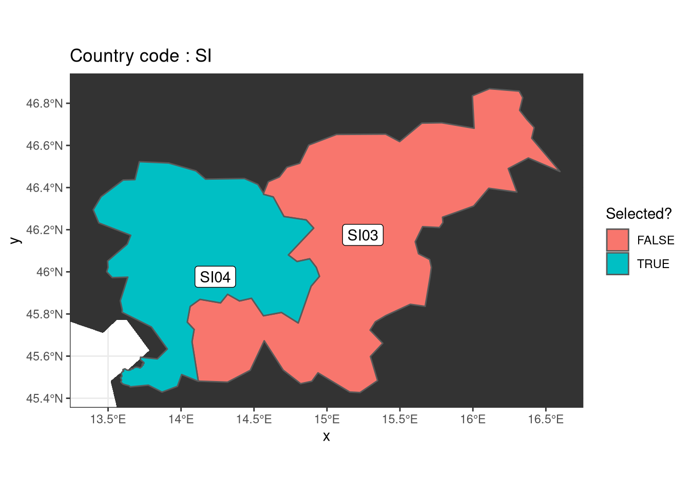
## Simple feature collection with 69 features and 6 fields
## geometry type: MULTIPOLYGON
## dimension: XY
## bbox: xmin: -24.31733 ymin: 34.57181 xmax: 34.39352 ymax: 71.15304
## epsg (SRID): 4326
## proj4string: +proj=longlat +datum=WGS84 +no_defs
## # A tibble: 69 x 7
## # Groups: CNTR_CODE [15]
## LEVL_CODE NUTS_ID CNTR_CODE NUTS_NAME FID geometry is.sel
## * <int> <fct> <chr> <fct> <fct> <MULTIPOLYGON [°]> <fct>
## 1 2 MT00 MT Malta MT00 (((14.35142 35.9738, 14.… TRUE
## 2 2 BE23 BE Prov. Oos… BE23 (((4.30783 51.12503, 4.1… TRUE
## 3 2 BE24 BE Prov. Vla… BE24 (((4.78932 51.03893, 4.8… TRUE
## 4 2 BE25 BE Prov. Wes… BE25 (((3.46031 50.7659, 3.32… TRUE
## 5 2 BE31 BE Prov. Bra… BE31 (((5.01957 50.75076, 4.9… TRUE
## 6 2 BE32 BE Prov. Hai… BE32 (((3.77568 50.74789, 3.8… TRUE
## 7 2 BE33 BE Prov. Liè… BE33 (((5.81905 50.71456, 5.8… TRUE
## 8 2 BE34 BE Prov. Lux… BE34 (((5.72155 50.26199, 5.8… TRUE
## 9 2 BE35 BE Prov. Nam… BE35 (((5.22126 50.4173, 5.30… TRUE
## 10 2 BG31 BG Северозап… BG31 (((22.99717 43.80787, 23… FALSE
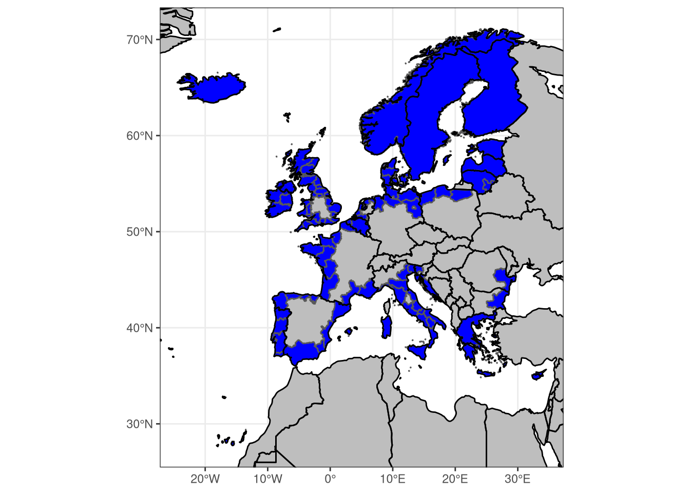
## # … with 59 more rowsThe final full set of “regions” for further analysis can be seen below.
3.5.2 Regional hazard
Calculating a regional climate-hazard score requires information about the fisheries and landings at this spatial scale. Due the fact that we are basing this risk analysis and our hazard definition on stocks, rather than species, this implies that we need not just information about the composition of landings in each region, but also the fishing area (FAO Subarea) where these fish were caught. We have two sources of information that approach this level of detail. The EUMOFA catch data gives species composition at the harbour level (which can then be aggregated into NUTS2 regions), but there is no indication where these fish were caught, making it difficult to link up to a stock. Alternatively, the “EUROSTAT catch” data provides catches by species and fishing region, but is only resolved at the national level.
We therefore need to infer the distribution of stocks making up the landings of that species in that region region. We make the assumption that the landings in each region come from the waters (specifically the FAO subregion) immediately adjacent. For example, a harbour fronting on to the North Sea will see landings of North Sea cod and herring, rather than Barents Sea cod and Norwegian Sea herring. Matching up the terrestial regions with the nearest stocks allows the stock composition for each species in a region to be set, and therefore the regional hazard calculated.
We can test the validity of this assumption using an internal consistency test. The “EUROSTAT catch” database provides the catch per country from each stock. If this assumption is corect, then these per stock catches should in principle match the total landings per species and FAO subarea when summed across all regions. Differences between the two will arise from stocks further away being landed in a region i.e. non adjacent regions, but also from discards, misreporting and general inconsistencies between the EUMOFA and EUROSTAT datasets.
The results of this internal consistency check are shown in the Supplementary material, and how that there is reasonable correlation (R=0.83) between these two metrics, supporting the validity of our assumption. In the end it may not be all that important because the only thing that varies by region (stock) is the safety margin and that of course is highly correlated in space so it may not matter at the end of the day.
3.5.3 Regional exposure
Following the approach applied to the fleet segments, Shannon diversity indices (H) and Simpson’s dominance indices (D) were then calculated for each NUTS2 region, and the combined metric used as measures of regional exposure.
3.5.4 Regional vulnerability
Metrics
3.5.5 Regional risk
- Combination
- Visualisations