Chapter 1 Introduction to Data
1.1 Chapter Overview
What is statistics? There are two ways to think about this:
- Facts and data, organized or summarized in such a way that they provide useful information about something.
- The science of analyzing, organizing, and summarizing data.
As a field, Statistics provides tools for scientists, practitioners, and laypeople to better understand data. You may find yourself using knowledge from this course in a research lab, while reading a research report, or even while watching the news!
Chapter Learning Objectives/Outcomes
After completing Chapter 1, you will:
- Understand basic statistical terminology.
- Produce data using sampling and experimental design techniques.
- Organize and visualize data using techniques for exploratory data analysis.
- Identify the shape of a data set.
- Understand and interpret graphical displays.
R objectives
- Manually enter data.
- Generate random numbers.
- Create histograms.
This chapter’s outcomes correspond to course outcomes (1) organize, summarize, and interpret data in tabular, graphical, and pictorial formats and (2) organize and interpret bivariate data and learn simple linear regression and correlation.
1.2 Statistics Terminology
There are two ways to think about statistics:
- Descriptive statistics are methods for describing information.
For example, 66% of eligible voters voted in the 2020 presidential election (the highest turnout since 1900!).
- Inferential statistics are methods for drawing inference (making decisions about something we are uncertain about).
For example, a poll suggests that 75% of voters will select Candidate A. People haven’t voted yet, so we don’t know what will happen, but we could reasonably conclude that Candidate A will win the election.
Data is factual information. We collect data from a population, the collection of all individuals or items a researcher is interested in.
- Collecting data from an entire population is called a census.
- This is complicated and expensive! There’s a reason the United States only does a census every 10 years.
- We can also take a sample, a subset of the population we get data from.
- If you think of the population as a pie, the sample is a small slice. Whether it’s a pumpkin pie, a cherry pie, or a savory pie, the small slice will tell you that. We don’t need to eat the entire pie to learn a lot about it!
Data are often organized in what we call a data matrix. If you’ve ever seen data in a spreadsheet, that’s a data matrix!
| Age | Gender | Smoker | Marital Status | |
| Person 1 | 45 | Male | yes | married |
| Person 2 | 23 | Female | no | single |
| Person 3 | 36 | Other | no | married |
| Person 4 | 29 | Female | no | single |
Each row (horizontal) represents one observation (also called observational units, cases, or subjects). These are the individuals or items in the sample.
Each column (vertical) represents a variable, the characteristic or thing being measured. Think of variables as measurements that can vary from one observation to the next.
There are two types of variable:
- Numeric or quantitative variables take numeric values AND it is sensible to do math with those values.
- Discrete numeric variables take numeric values with jumps. Typically, this means they can only take whole number values. These are often counts of something - for example, counting the number of pets you have.
- Continuous numeric variables take values “between the jumps”. Typically, this means they can take decimal values.
- Categorical or qualitative variables take values that are categories.
- Sometimes, categories can be represented by numbers. Ask yourself if it makes sense to do math with those numbers. If it doesn’t make sense, it’s probably a categorical variable. (Ex: zip codes)
- If you’re unsure whether a variable is discrete or continuous, pick a number with some decimal places - like 1.83 - and ask yourself if that value makes sense. If it doesn’t, it’s probably discrete. (Ex: number of siblings)
R: Entering Data
We can work with data in R by reading it in from a file or by entering it manually. To enter numeric data manually, we use the c command.
The following line of code saves the age data from the data matrix example above:
age = c(45, 23, 36, 29)Notice that we set age equal to c() with the numbers in the parentheses, separated by commas. Also notice that the numbers are in the same order as in the data. If I want to use the age variable later, I can refer to it directly in R and it will print out the values in that variable:
age = c(45, 23, 36, 29)To enter categorical data in R, we do the same thing, but with the addition of quotation marks:
gender = c("Male", "Female", "Other", "Female")Section Exercises
The following table shows part of the data matrix from a Stat 1 course survey.
| Age | Year in college | What is your major? | Units this semester | |
| 1 | 19 | Sophomore | Health Sciences | 15 |
| 2 | 19 | Sophomore | Business | 15 |
| 3 | 19 | Sophomore | Undecided | 14 |
| \(\vdots\) | \(\vdots\) | \(\vdots\) | \(\vdots\) | \(\vdots\) |
| 29 | 21 | Junior | Business | 15 |
What does each row of the data matrix represent?
What does each column of the data matrix represent?
Indicate whether each variable is discrete numeric, continuous numeric, or categorical.
Dig Deeper
Read the article, Here’s Why an Accurate Census Count Is So Important from the New York Times. (If you can’t access the article, try a Google search for “why an accurate census count is important”.) Take a moment to write down your thoughts on the relationship between how we collect data (for example - the questions asked in the census) and the power data has over people’s lives. As researchers, scientists, and consumers of media, what are some reasons this is important to think about?
1.3 Sampling and Design
1.3.1 Statistical Sampling
How do we get samples? We want a sample that represents our population. Representative samples reflect the relevant characteristics of our population.
In general, we get representative samples by selecting our samples at random and with an adequate sample size.
A non-representative sample is said to be biased. For example, if we used a sample of chihuahuas to represent all dogs, we probably wouldn’t get very good information; that sample would be biased.
These can be a result of convenience sampling, choosing a sample based on ease.
In our daily lives, common sources of bias are anecdotal evidence and availability bias. Anecdotal evidence is data based on personal experience or observation. Typically this consists of only one or two observations and is NOT representative of the population.
Example: anecdotal evidence. A friend tells you their grandpa smoked a pack of cigarettes a day and lived to be 100. Does this mean that cigarettes will help you live to 100? no!
Availability bias is your brain’s tendency to think that examples of things that come readily to mind are more representative than is actually the case.
Example: availability bias. Shark attacks are actually extremely uncommon, but the media tends to report on extreme anecdotes, making us more prone to this kind of bias!
We avoid bias by taking random samples. One type of random sample is a simple random sample. We can think of this as “raffle sampling”, like drawing names out of a hat. Each case (or each possible sample) has an equal chance of being selected. Knowing that A is selected doesn’t tell us anything about whether B is selected. Instead of literally drawing from a hat, we usually use a random number generator from a computer.
1.3.2 Experimental Design
When we do research, we have two options:
- Conduct an experiment, where researchers assign treatments to cases.
- Treatments are experimental conditions.
- In an experiment, cases may also be called experimental units (items or individuals on which the experiment is performed).
- Conduct an observational study, where no conditions are assigned. These are often done for ethical reasons, like examining the impacts of smoking cigarettes.
Experiments allow us to infer causation. Observational studies do not.
Experimental design principles:
- Control: two or more treatments are compared.
- Randomization: experimental units are assigned to treatment groups (usually and preferably at random).
- Replication: a large enough sample size is used to test each treatment many times (on many different experimental units).
- Blocking: if variables other than treatment are likely to have an impact on study outcome, we use blocks.
- For example, I might separate patients in a medical study into “high risk” and “low risk” blocks. I would randomly assign all of the high risk patients to a treatment and then randomly assign all of the low risk patients to a treatment. This helps ensure an even distribution of high/low risk patients in each treatment group.
An experiment without blocking has a completely randomized design; an experiment with blocking has a randomized block design.
In an experimental setting, we talk about
- Response variable: the characteristic of the experimental outcome being measured or observed.
- Factor: a variable whose impact on the response variable is of interest in the experiment.
- Levels: the possible values of a factor.
- Treatments: experimental conditions (based on combinations of factor levels).
In human subjects research, we do a little extra work:
- If subjects do not know what treatment group they are in, the study is called blind.
- We use a placebo (fake treatment) to achieve this.
- If neither the subjects nor the researchers who interact with them know the treatment group, it is called double blind.
This helps avoid bias caused by placebo effect, doctor’s expectations for outcome, etc.!
R: Random Number Generation
To generate a random whole number using R, we can use the sample command. We use the sample command like sample(minimum:maximum, size = n), replacing minimum with the minimum value (often the number 1), maximum with the maximum value, and n with the sample size.
The following command takes a random sample of size 1 from the values 1 through 10 (the numbers 1, 2, 3, 4, 5, 6, 7, 8, 9, 10):
sample(1:10, size = 1)## [1] 1Section Exercises
A group of researchers wanted to know if puppies had an effect on heart rate. From a sample of 18 people, they had 10 take a test while in a room with a puppy. The remaining 8 people took the same test in a room with no puppies.
Is this an observational study or an experiment? Explain.
Identify the (i) cases and (ii) response variable.
1.4 Frequency Distributions
1.4.1 Qualitative Variables
Frequency (count): the number of times a particular value occurs.
A frequency distribution lists each distinct value with its frequency.
| Class | Frequency |
|---|---|
| freshman | 12 |
| sophomore | 10 |
| junior | 3 |
| senior | 5 |
A bar plot is a graphical representation of a frequency distribution. Each bar’s height is based on the frequency of the corresponding category.
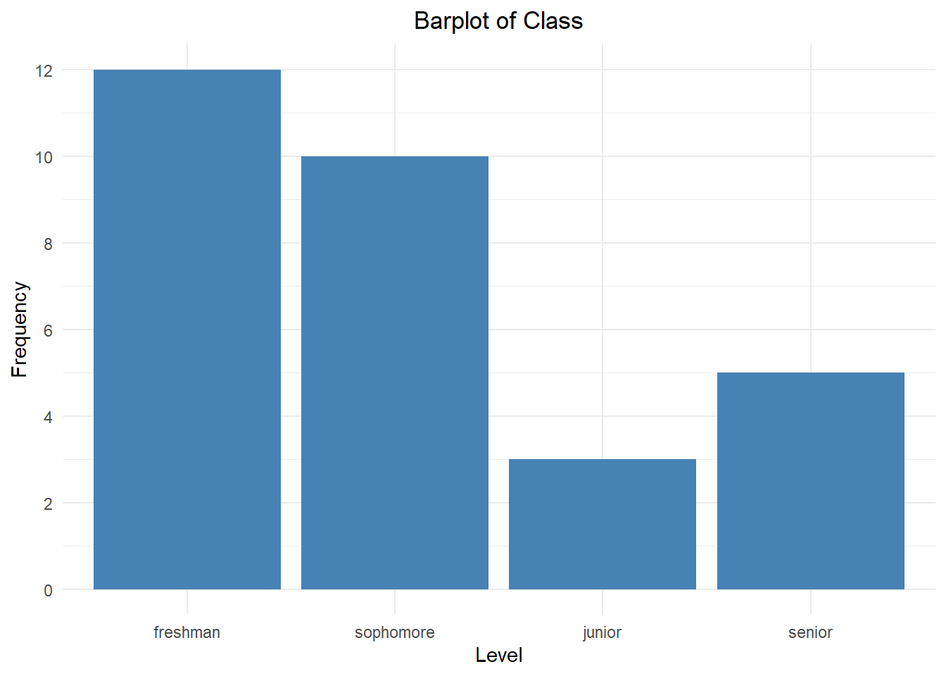
The bar plot above shows the class level breakdown for students in an Introductory Statistics course. Take a moment to notice how the bars match up with the frequency distribution above.
Relative frequency is the ratio of the frequency to the total number of observations.
\[ \text{relative frequency} = \frac{\text{frequency}}{\text{number of observations}} \]
This is also called the proportion. The percentage can be obtained by multiplying the proportion by 100.
A relative frequency distribution lists each distinct value with its relative frequency.
| Class | Frequency | Relative Frequency | Percent |
|---|---|---|---|
| freshman | 12 | \(12/30 = 0.4\) | 40% |
| sophomore | 10 | \(10/30 \approx 0.3333\) | 33.33% |
| junior | 3 | \(3/30 = 0.1\) | 10% |
| senior | 5 | \(5/30 \approx 0.1667\) | 16.67% |
1.4.2 Quantitative Variables
We can also apply this concept to numeric data. A dot plot is one graphical representation of this. A dot plot shows a number line with dots drawn above the line. Each dot represents a single point.
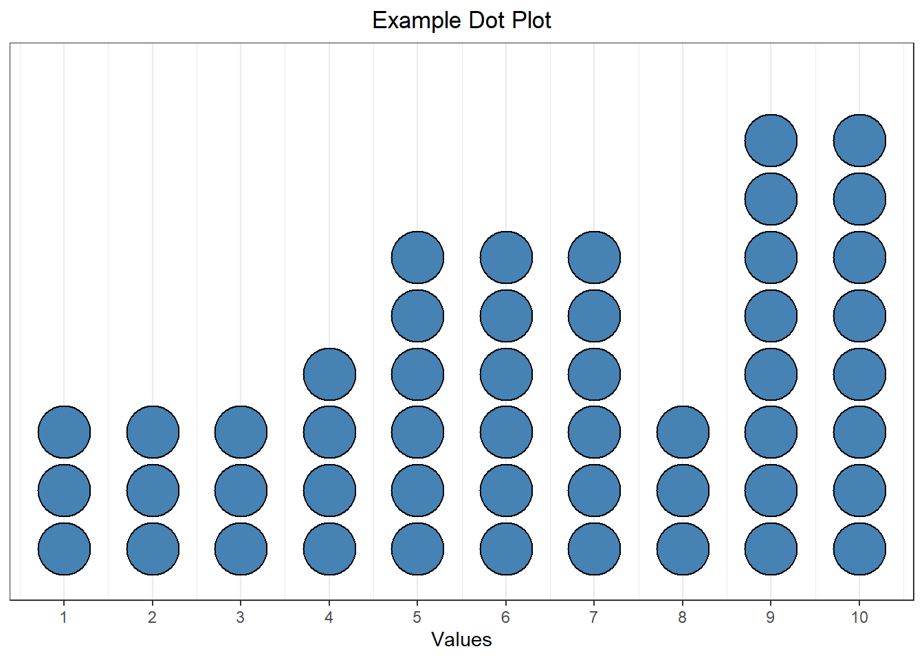
For example, the dot plot above shows a sample where the value 1 appears three times, the value 5 appears six times, etc.
We would also like to be able to visualize larger, more complex data sets. This is hard to do using a dot plot! Instead, we can do this using bins, which group numeric data into equal-width consecutive intervals.
Example: A random sample of weights (in lbs) from 12 cats:
\[\quad 6.2 \quad 11.6 \quad 7.2 \quad 17.1 \quad 15.1 \quad 8.4 \quad 7.7 \quad 13.9 \quad 21.0 \quad 5.5 \quad 9.1 \quad 7.3 \]
The minimum (smallest value) is 5.5 and the maximum (largest value) is 21. There are lots of ways to break these into “bins”, but what about…
- 5 - 10
- 10 - 15
- 15 - 20
- 20 - 25
Each bin has an equal width of 5, but if we had a cat with a weight of exactly 15 lbs, would we use the second or third bin?? It’s unclear. To make this clear, we need there to be no overlap. Instead, we could use:
Weight Count 5 - <10 7 10 - <15 2 15 - <20 2 20 - <25 1 Now, a cat with a weight of 15.0 lbs would be placed in the third bin (but not the second).
We will visualize this using a histogram, which is a lot like a bar plot but for numeric data:
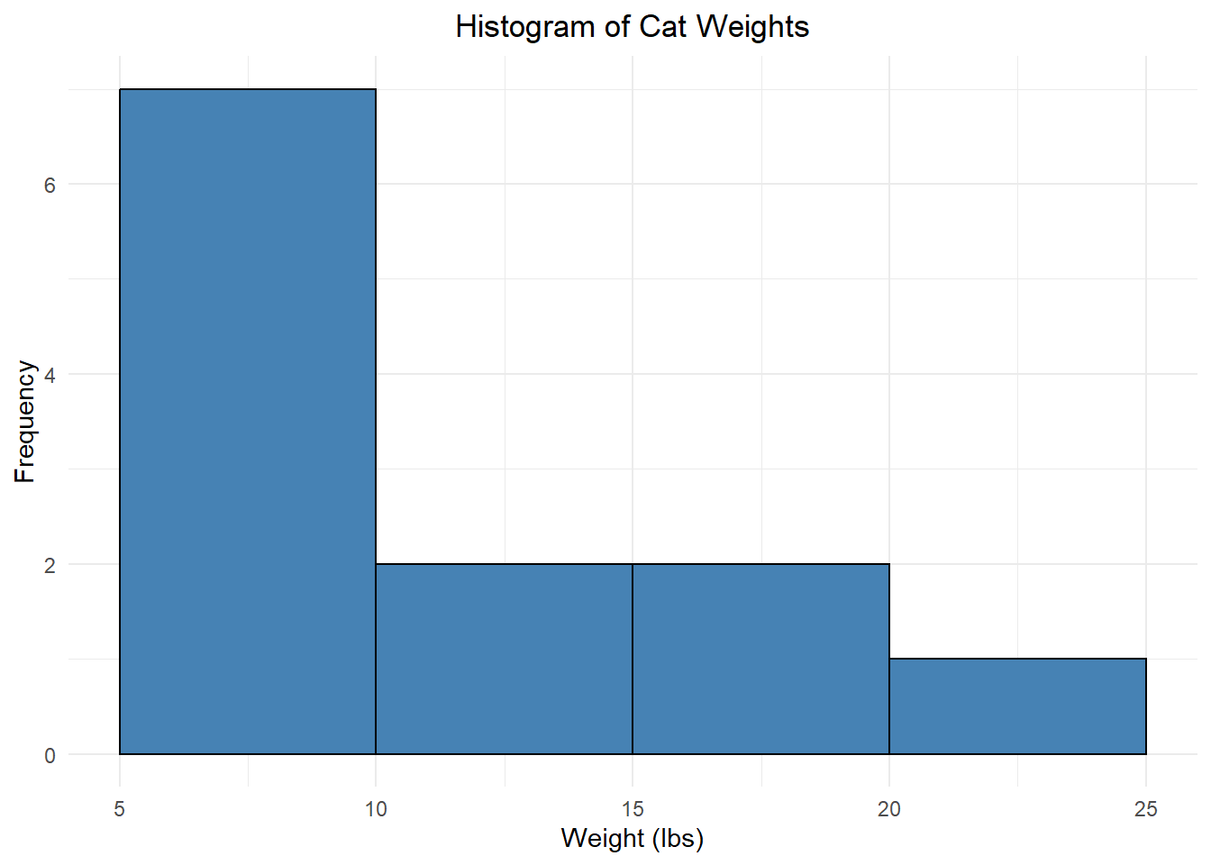
This is what we call a frequency histogram because each bar height reflects the frequency of that bin. We can also create a relative frequency histogram which displays the relative frequency instead of the frequency:
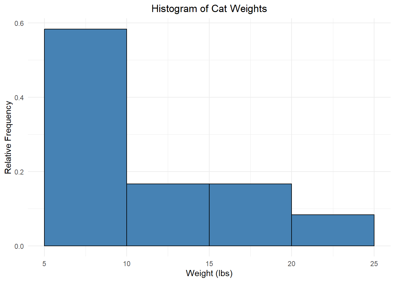
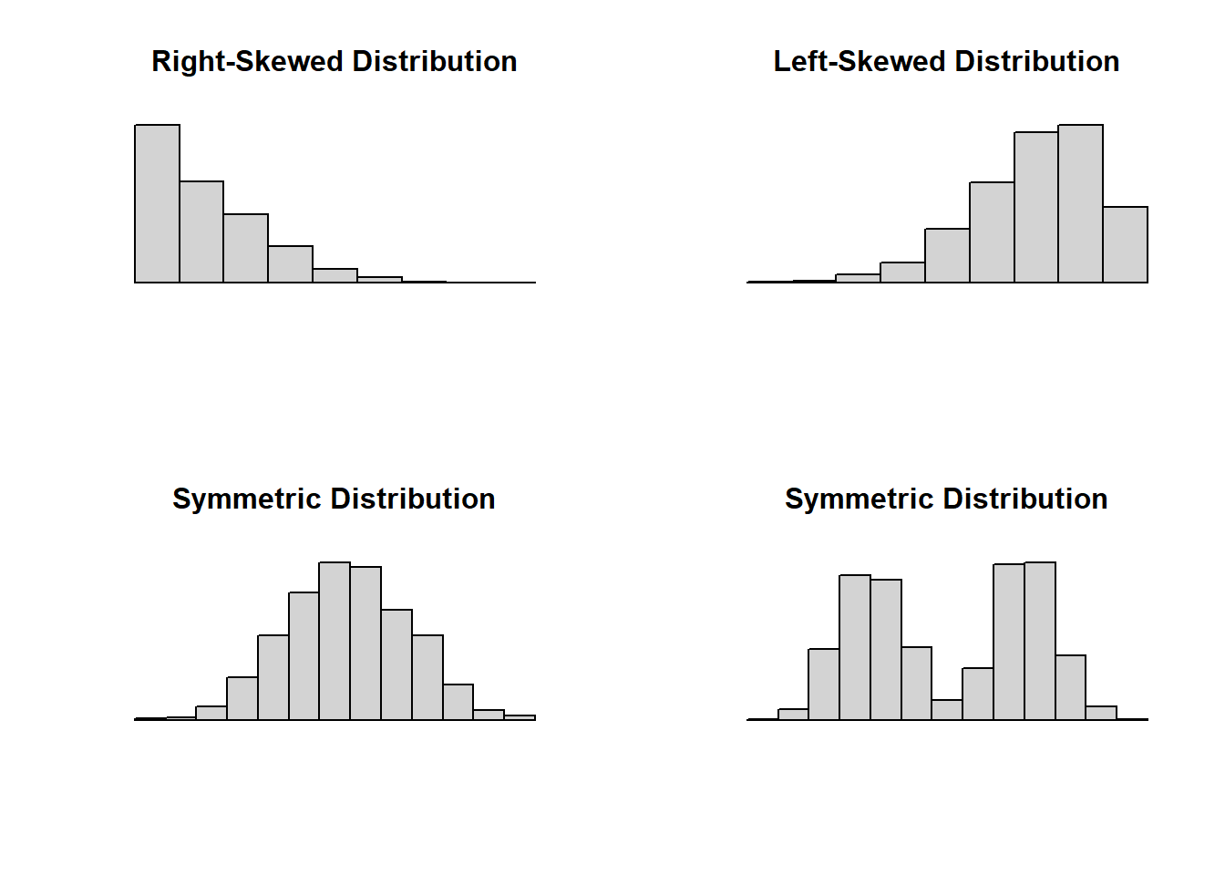
Notice that these last two histograms look the same except for the numbers on the vertical axis! This gives us insight into the shape of the data distribution, literally how the values are distributed across the bins. The part of the distribution that “trails off” to one or both sides is called a tail of the distribution.
When a histogram trails off to one side, we say it is skewed (right-skewed if it trails off to the right, left-skewed if it trails off to the left). Data sets with roughly equal tails are symmetric.
We can also use a histogram to identify modes. For numeric data, especially continuous variables, we think of modes as prominent peaks.
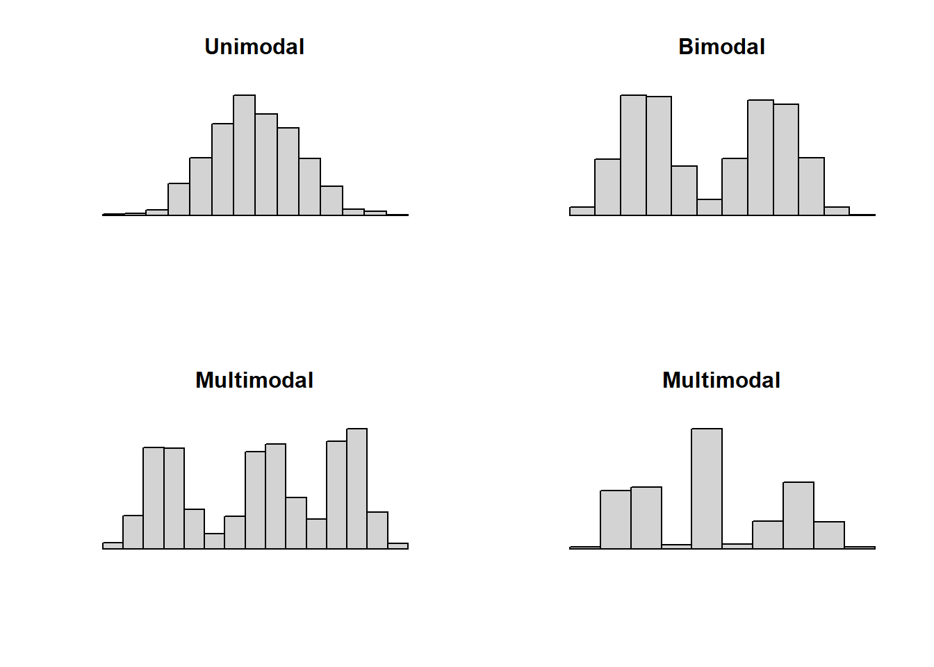
- Unimodal: one prominent peak.
- Bimodal: two prominent peaks.
- Multimodal: three or more prominent peaks.
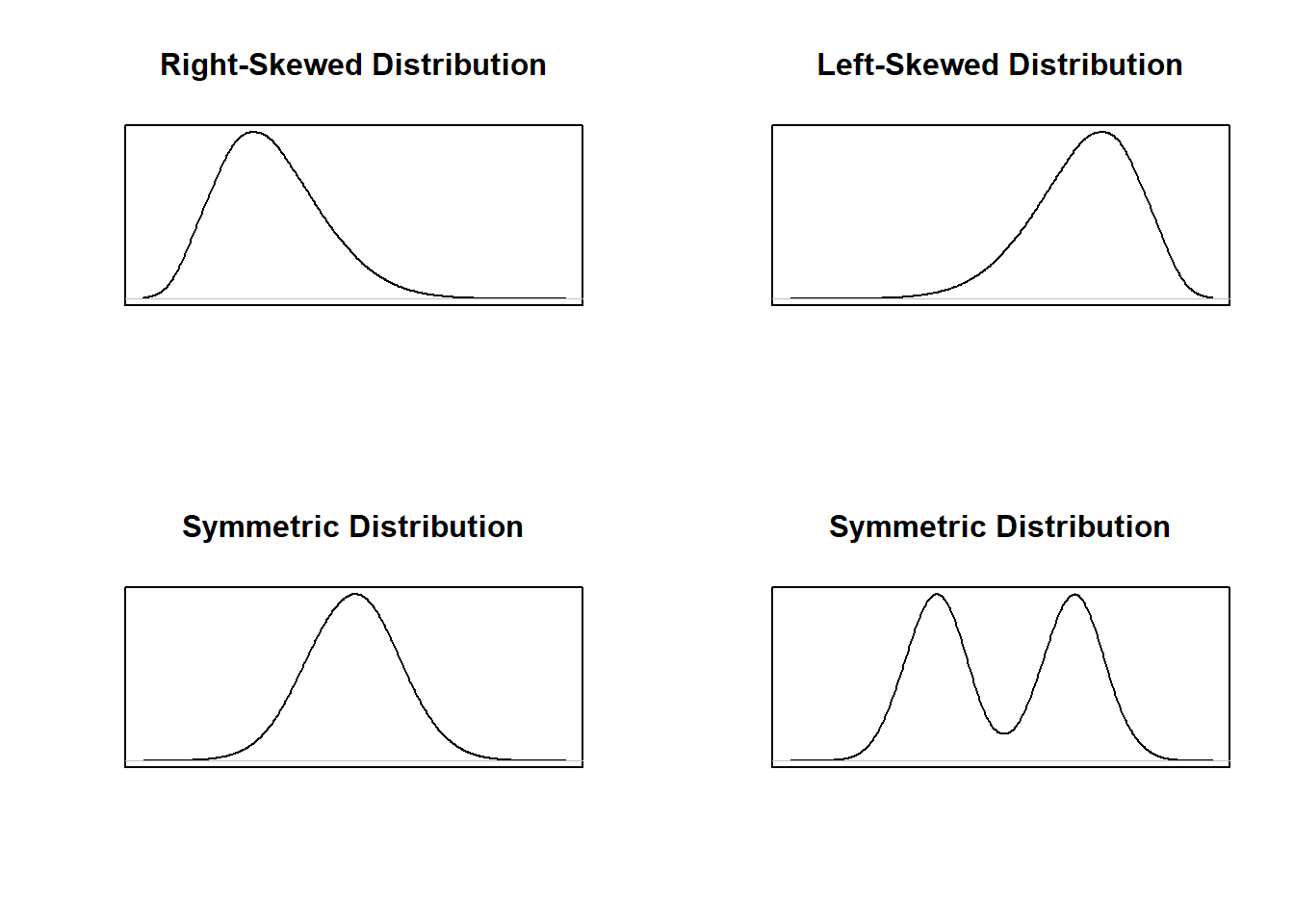
Finally, we can also “smooth out” these histograms and use a smooth curve to examine the shape of the distribution. Below are the smooth curve versions of the distributions shown in the four histograms used to demonstrate skew and symmetry.
R: Histograms
There is a built-in dataset in R called Loblolly, which contains the variables height and age of some Loblolly pine trees. I can refer to this data by typing in Loblolly directly. To view just the first few observations (out of the 84 total in the data), I can use the head command:
head(Loblolly)## height age
## 1 4.51 3
## 2 10.89 5
## 3 28.72 10
## 4 41.74 15
## 5 52.70 20
## 6 60.92 25The information that appears next to each ## is what R prints out for us.
In order to refer to the variables in Loblolly directly, I will need to use the attach command. This tells R that when I say age I mean the age variable from the Loblolly dataset (and not from some other dataset).
I want to create a histogram to visualize the ratio of tree height to age. First, I need to find this ratio for each observation. I can do this easily in R by dividing height by age. I will save this as a new variable called htage_ratio.
htage_ratio = height/ageThen to create a histogram of the height to age ratio, we will use the command hist on the variable htage_ratio:
hist(htage_ratio)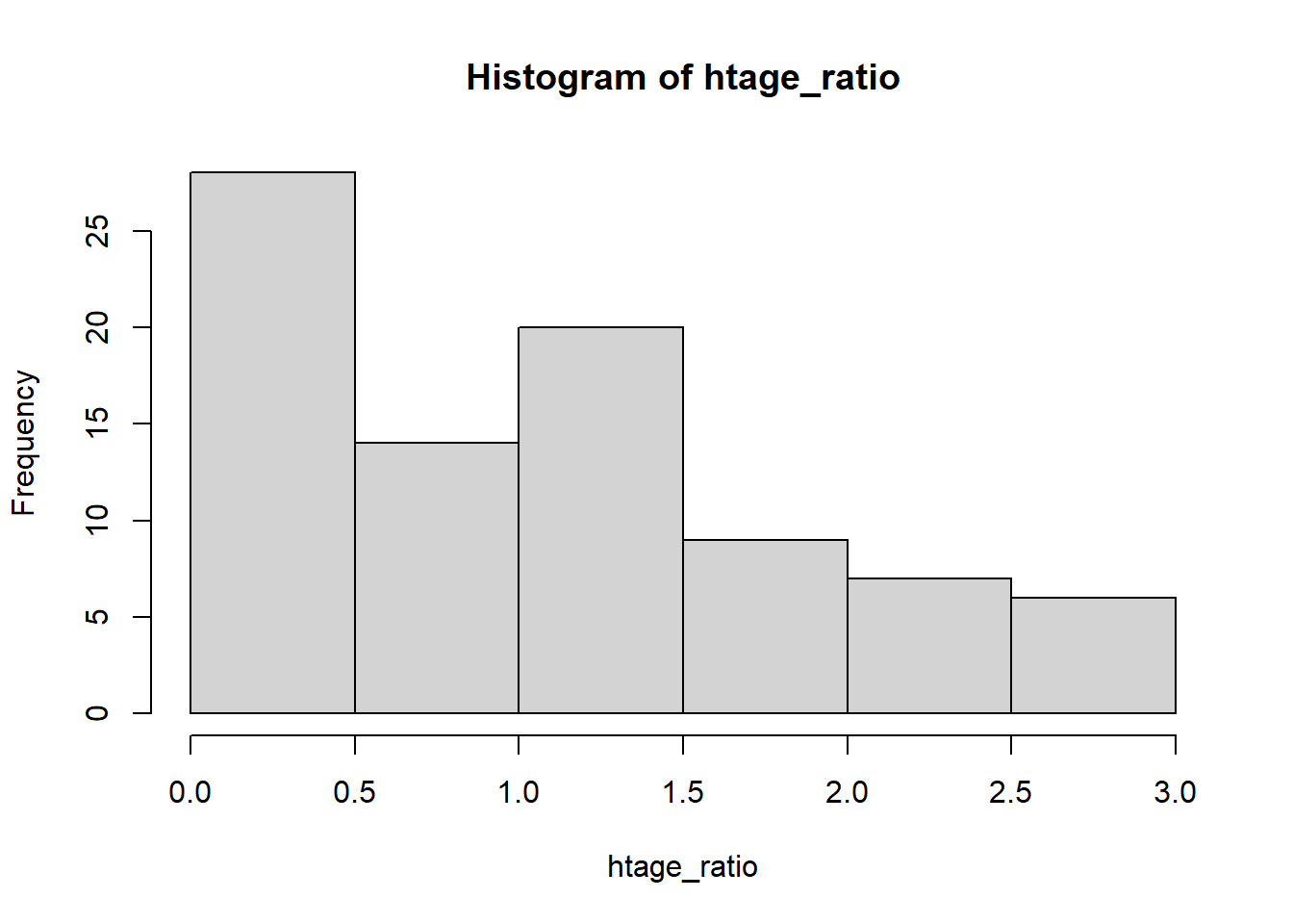
I can clean up this graph by taking advantage of additional arguments in the hist command:
mainis where I can give the plot a new title. (Make sure to put the title in quotes!)xlabis the x-axis (horizontal axis) title.ylabis the y-axis (vertical axis) title.freqallows us to create either frequency or relative frequency histograms.- If we set it equal to
TRUEit will produce a frequency histogram. (This is the default if we don’t give R any instructions.) - If we set it equal to
FALSEit will produce a relative frequency histogram.
- If we set it equal to
colallows us to give R a specific color for the bars.
Notice that each argument is separated by a comma.
hist(htage_ratio,
     main = "Histogram of Height-to-Age Ratio",
     xlab = "Height-to-Age Ratio (feet/year)",
     ylab = "Relative Frequency",
     freq = FALSE,
     col = 'pink')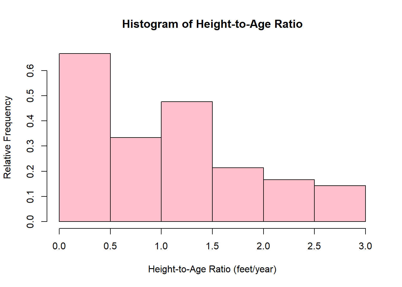
When I am done, I will use the detatch command to tell R that I am not working with the Loblolly data anymore.
detach(Loblolly)