Appendices
Appendix B: Average Deviance
The deviance of an observation from its mean is \(x - \bar{x}\). We denote the deviation for the \(i\)th observation as \(x_i - \bar{x}\). So the sum over all \(n\) deviances is
\[\begin{align} \text{Sum of Deviances} &= \Sigma_{i=1}^n (x_i - \bar{x}) \\ &= (x_1 - \bar{x}) + (x_2 - \bar{x}) + \dots + (x_{n-1} - \bar{x}) + (x_n - \bar{x}) \\ &= x_1 - \bar{x} + x_2 - \bar{x} + \dots + x_{n-1} - \bar{x} + x_n - \bar{x} \\ &= x_1 + x_2 + \dots + x_{n-1} + x_n - \bar{x} - \bar{x} - \dots - \bar{x} - \bar{x} \\ &= (x_1 + x_2 + \dots + x_{n-1} + x_n) - (\bar{x} + \bar{x} + \dots + \bar{x} + \bar{x}) \end{align}\]
where the first half is the sum over all of the \(x\) values and the term (\(\bar{x}\)) appears \(n\) times. So we can rewrite this as
\[ \text{Sum of Deviances} = \Sigma_{i=1}^n (x_i) - n\bar{x} \] Now notice that, because \(\bar{x} = \frac{\Sigma_{i=1}^n (x_i)}{n}\), we can multiply both sides by \(n\) to get \(n\bar{x} = \Sigma_{i=1}^n (x_i)\) and rewrite the sum over the deviances as
\[\begin{align} \text{Sum of Deviances} &= n\bar{x} - n\bar{x} \\ &=0 \end{align}\]
Appendix C: Deriving a Confidence Interval
Assume we are taking a sample from a normal distribution with mean \(\mu\) and standard deviation \(\sigma\). We will assume the value of \(\sigma\) is known to us. Then \(\bar{X}\) is Normal(\(\mu, \sigma/\sqrt{n}\)). If we standardize \(\bar{X}\), we get \[Z = \frac{\bar{X}-\mu}{\sigma/\sqrt{n}}.\]
We want some interval \((a,b)\). We will start by considering \(a < Z < b\), so \(a < Z\) and \(Z < b\) (or \(b > Z\)). Then
\[ \begin{aligned} Z &< b\\ \frac{\bar{X}-\mu}{\sigma/\sqrt{n}} &< b\\ \bar{X}-\mu &< b\sigma/\sqrt{n} \\ \bar{X}-b\sigma/\sqrt{n} &< \mu \end{aligned} \]
and
\[ \begin{aligned} a &< Z \\ a &< \frac{\bar{X}-\mu}{\sigma/\sqrt{n}} \\ a\sigma/\sqrt{n} &< \bar{X}-\mu \\ \mu &< \bar{X}-a\sigma/\sqrt{n} \end{aligned} \]
putting these together, \[ \bar{X}-b\frac{\sigma}{\sqrt{n}} < \mu < \bar{X}-a\frac{\sigma}{\sqrt{n}}.\] If we want to be 95% confident, then we want \(P(a < Z < b)=0.95\): \[P\left(\bar{X}-b\frac{\sigma}{\sqrt{n}} < \mu < \bar{X}-a\frac{\sigma}{\sqrt{n}}\right) = 0.95.\] To calculate the 95% confidence interval, we need to find \(a\) and \(b\) such that \(P(a < Z < b)=0.95\).
We want this interval to be as narrow (small) as possible. Why? Narrower intervals are more informative. If I say I’m 95% confident that tomorrow’s high will be between -100 and 200 degrees Fahrenheit, that’s a useless interval. If I change it to between 70 and 100, that’s a little better. Changing it to between 85 and 90 is even better. This is what we mean by more informative.
It turns out that with a symmetric distribution like the normal distribution, the way to make a confidence interval as narrow as possible is to take advantage of this symmetry. Each of the plots below show a shaded area of 0.95. The narrowest interval (along the horizontal axis) is the first interval, which is shaded on \((-1.96 < Z < 1.96)\).
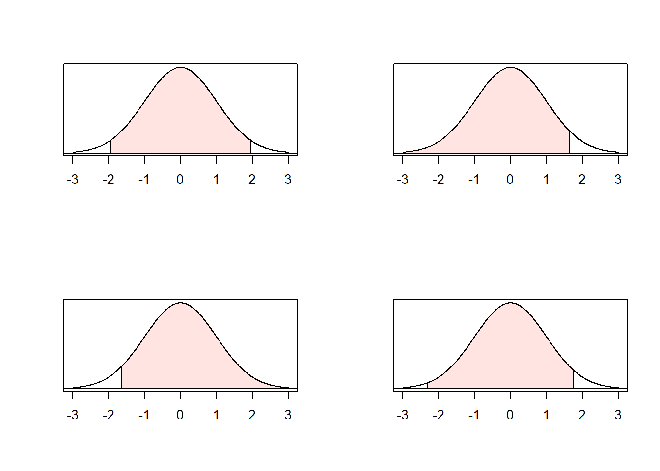
Using the symmetry of the normal distribution, we find that the narrowest interval uses \(a = -1.96\) and \(b = 1.96\), which results in the 95% confidence interval \[\left(\bar{x} - z_*\frac{\sigma}{\sqrt{n}}, \bar{x} + z_*\frac{\sigma}{\sqrt{n}}\right)\] where \(z_* = 1.96\).