Chapter 2 Descriptive Measures

2.1 Chapter Overview

In the previous chapter, we thought about descriptive statistics using tables and graphs. Next, we summarize data by computing numbers. Some of these numbers you may already be familiar with, such as averages and percentiles. Numbers used to describe data are called descriptive measures.

Chapter Learning Objectives/Outcomes

After completing Chapter 2, you will be able to:

Calculate and interpret measures of center.
Calculate and interpret measures of variation.
Find and interpret measures of position.
Summarize data using boxplots.

R objectives

Generate measures of center.
Generate measures of variability.
Generate measures of position.
Create box plots.

This chapter’s outcomes correspond to course outcomes (1) organize, summarize, and interpret data in tabular, graphical, and pictorial formats, (2) organize and interpret bivariate data and learn simple linear regression and correlation, and (6) apply statistical inference techniques of parameter estimation such as point estimation and confidence interval estimation.

2.2 Measures of Central Tendency

One research question we might ask is : what values are most common or most likely?

Mode: the most commonly occurring value. We can use this for numeric variables, but typically we use the mode when talking about categorical data.

Mean: this is what we usually think of as the “average”. Denoted \(\bar{x}\). Add up all of the values and divide by the number of observations (\(n\)): \[ \bar{x} = \frac{x_1 + x_2 + \dots + x_n}{n} = \sum_{i=1}^n \frac{x_i}{n} \] where \(x_i\) denotes the \(i\)th observation and \(\sum_{i=1}^n\) is the sum of all observations from 1 through \(n\). This is called summation notation.

Median: the middle number when the data are ordered from smallest to largest.

If there are an odd number of observations, this will be the number in the middle: {1, 3, 7, 9, 9} has median 7
If there are an even number of observations, there will be two numbers in the middle. The median will be their average. {1, 2, 4, 7, 9, 9} has median \(\frac{4+7}{2}=5.5\)

The mean is sensitive to extreme values and skew. The median is not!

	\(x\): 1, 3, 7, 9, 9	\(y\): 1, 3, 7, 9, 45
Median	\(\text{median} = 7\)	\(\text{median} = 7\)
Mean	\(\bar{x} = \frac{29}{5} = 5.8\)	\(\bar{y} = \frac{65}{5} = 13\)

Notice how changing that 9 out for a 45 changes the mean a lot! But the median is 7 for both \(x\) and \(y\).

Because the median is not affected by extreme observations or skew, we say it is a resistant measure or that it is robust.

Which measure should we use?

Mean: symmetric, numeric data
Median: skewed, numeric data
Mode: categorical data

Note: If the mean and median are roughly equal, it is reasonable to assume the distribution is roughly symmetric.

R: Finding Measures of Center

To find a mean in R, we use the command mean. Let’s use the Loblolly pine data again and find the mean tree height.

attach(Loblolly)
mean(height)

## [1] 32.3644

From R, we can see that the sample mean height of the Loblolly pines is 32.36 feet. (Note that R will often print things out with ## and a number in square brackets. This is just to help us keep track of things if we write a lot of lines of code. You can ignore that number in the brackets!)

Is a mean the appropriate measure of center? We can quickly check the skew with a histogram:

hist(height)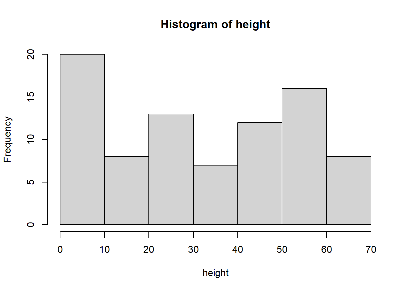

It might be a little bit hard to tell with this histogram, but it does not look particularly skewed. Let’s use our other trick: if the mean and median are approximatly equal, we can say the distribution is approximately symmetric (and therefore the mean is an appropriate measure of center). To calculate the median, we use the command median:

## [1] 34

The sample median of the Loblolly pine heights is 34 feet. Since the mean and median are approximately equal, it would be reasonable to use the mean in this case. To find a mode (for a categorical variable), we would repeat the same process but with the command mode.

2.3 Measures of Variability

How much do the data vary?

Should we care? Yes! The more variable the data, the harder it is to be confident in our measures of center!

If you live in a place with extremely variable weather, it is going to be much harder to be confident in how to dress for tomorrow’s weather… but if you live in a place where the weather is always the same, it’s much easier to be confident in what you plan to wear.

We want to think about how far observations are from the measure of center.

One easy way to think about variability is the range of the data: \[\text{range} = \text{maximum} - \text{minimum}\] This is quick and convenient, but it is extremely sensitive to outliers! It also takes into account only two of the observations - we would prefer a measure of variability that takes into account all the observations.

Deviation is the distance of an observation from the mean: \(x - \bar{x}\). If we want to think about how far - on average - a typical observation is from the center, our intuition might be to take the average deviance… but it turns out that summing up the deviances will always result in 0! Conceptually, this is because the stuff below the mean (negative numbers) and the stuff above the mean (positive numbers) end up canceling each other out until we end up at 0. (If you are interested, Appendix A: Average Deviance has a mathematical proof of this using some relatively straightforward algebra.)

One way to deal with this is to make all of the numbers positive, which we accomplish by squaring the deviance.

	Deviance	Squared Deviance
\(x\)	\(x - \bar{x}\)	\((x - \bar{x})^2\)
2	-1.2	1.44
5	1.8	3.24
3	-0.2	0.04
4	0.8	0.64
2	-1.2	1.44
\(\bar{x}=3.2\)	Total = 0	Total = 6.8

Variance (denoted \(s^2\)) is the average squared distance from the mean: \[ s^2 = \frac{(x_1-\bar{x})^2 + (x_2-\bar{x})^2 + \dots + (x_n-\bar{x})^2}{n-1} = \frac{1}{n-1}\sum_{i=1}^n (x_i - \bar{x})^2 \] where \(n\) is the sample size. Notice that we divide by \(n-1\) and NOT by \(n\). There are some mathematical reasons why we do this, but the short version is that it’ll be a better estimate when we talk about inference.

Finally, we come to standard deviation (denoted \(s\)). \[s = \sqrt{s^2}\] The standard deviation is the square root of the variance. We say that a “typical” observation is within about one standard deviation of the mean (between \(\bar{x}-s\) and \(\bar{x}+s\)).

In practice (including in this class), we will use a computer to calculate the variance and standard deviation.

We will think about one more measure of variability, the interquartile range, in the next section.

R: Finding Measures of Variability

To find a range in R, we get started using the command range. Let’s keep using the Loblolly pine data again and find the mean tree height.

attach(Loblolly)

range(height)

## [1]  3.46 64.10

This command gives us the minimum and maximum values. Then to calculate the range, we would find \(64.10 - 3.46\). We can also do this in R, because R doubles as a calculator!

64.1 - 3.46

## [1] 60.64

The sample range of the Loblolly pine heights is 60.64 feet.

To find the variance and standard deviation, we use the commands var and sd, respectively:

var(height)

## [1] 427.3979

The sample variance of the Loblolly pine heights is 427.4.

sd(height)

## [1] 20.6736

detach(Loblolly)

The sample standard deviation of the Loblolly pine heights is 20.67 feet.

2.4 Measures of Position

The interquartile range (IQR) represents the middle 50% of the data.

Recall that the median cut the data in half: 50% of the data is below and 50% is above the median. This is also called the 50th percentile. The \(p\)th percentile is the value for which \(p\)% of the data is below it.

To get the middle 50%, we will split the data into four parts:

1	2	3	4
25%	25%	25%	25%

The 25th and 75th percentiles, along with the median, divide the data into four parts. We call these three measurements the quartiles:

Q1, the first quartile, is the median of the lower 50% of the data.
Q2, the second quartile, is the median.
Q3, the third quartile, is the median of the upper 50% of the data.

Example: Consider {1, 2, 3, 4, 5, 6, 7, 8, 9, 10}

Cutting the data in half: {1, 2, 3, 4, 5 | 6, 7, 8, 9, 10}, the median (Q2) is \(\frac{5+6}{2}=5.5\).

Q1 is the median of {1, 2, 3, 4, 5}, or 3

Q3 is the median of {6, 7, 8, 9, 10}, or 8

Note: this is a “quick and dirty” way of finding quartiles. A computer will give a more exact result.

Then the interquartile range is \[ \text{IQR} = \text{Q3}-\text{Q1} \]

This is another measure of variability and is resistant to extreme values. In general, we prefer the mean and standard deviation when the data are symmetric and we prefer the median and IQR when the data are skewed.

2.4.1 Box Plots

Our measures of position are the foundation for constructing what we call a box plot, which summarizes the data with 5 statistics plus extreme observations:

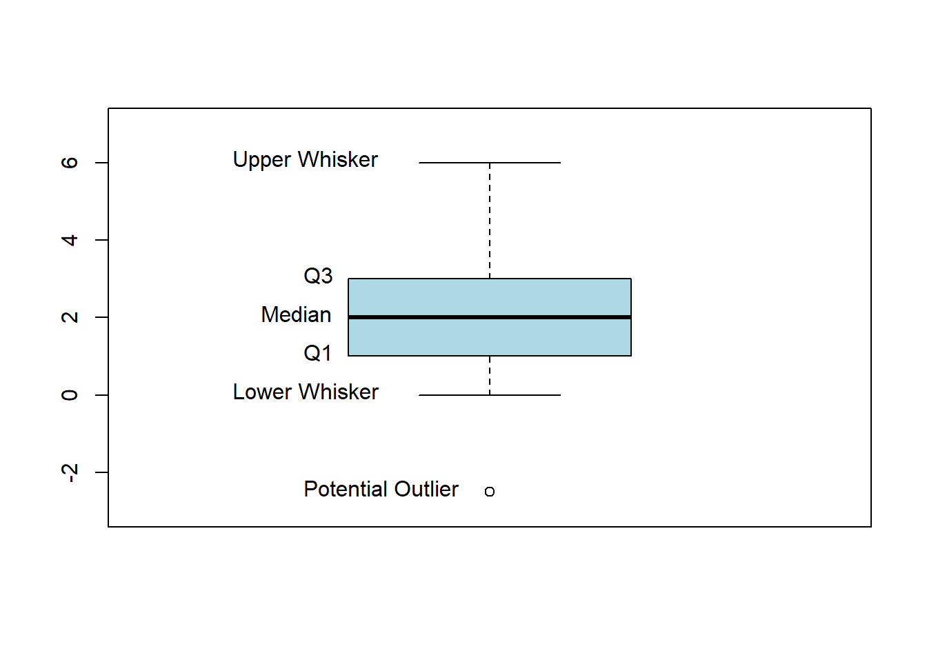
Drawing a box plot:

Draw the vertical axis to include all possible values in the data.
Draw a horizontal line at the median, at \(\text{Q1}\), and at \(\text{Q3}\). Use these to form a box.
Draw the whiskers. The whiskers’ upper limit is \(\text{Q3}+1.5\times\text{IQR}\) and the lower limit is \(\text{Q1}-1.5\times\text{IQR}\). The actual whiskers are then drawn at the next closest data points within the limits.
Any points outside the whisker limits are included as individual points. These are potential outliers.

(Potential) outliers can help us…

examine skew (outliers in the negative direction suggest left skew; outliers in the positive direction suggest right skew).
identify issues with data collection or entry, especially if the value of an outlier doesn’t make sense.

As with most things in this text, we won’t draw a lot of boxplots by hand. However, understanding how they are drawn will help us understand how to interpret them!

R: Measures of Position

Let’s continue using the Loblolly pine data.

attach(Loblolly)

We can get the quartiles quickly using the summary command. This will also give us the minimum, mean, and maximum. That’s fine!

summary(height)

##    Min. 1st Qu.  Median    Mean 3rd Qu.    Max. 
##    3.46   10.47   34.00   32.36   51.36   64.10

So \(Q1 = 10.46\), \(Q2 = \text{Median} = 34\), and \(Q3 = 51.35\). We can also quickly get the interquartile range using the IQR command.

IQR(height)

## [1] 40.895

detach(Loblolly)

R: Box Plots

attach(Loblolly)

To create a boxplot in R, we use the command boxplot. We can use some of the same arguments we used with the hist command to give it titles and color:

main is where I can give the plot a new title. (Make sure to put the title in quotes!)
ylab is the y-axis (vertical axis) title.
col allows us to give R a specific color for the bars. Notice that I also have to put the color in quotes.

boxplot(height,
        main = "Boxplot of Loblolly Pine Heights", 
        ylab = "Height (feet)",
        col = "green")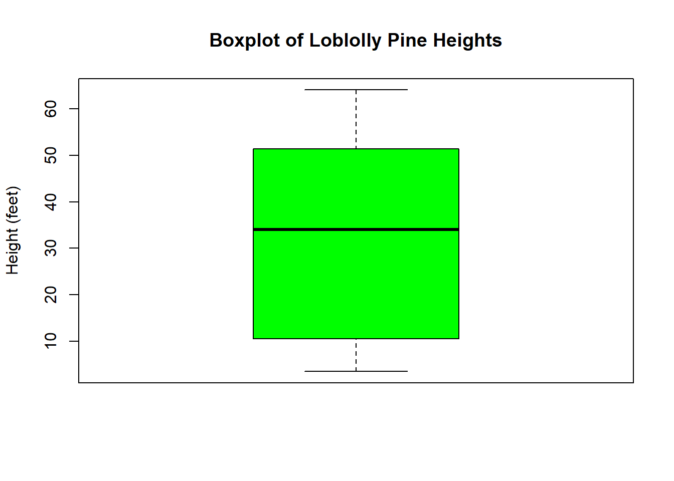

R will automatically create the entire box plot, including showing any outliers. (Which we should note that there aren’t any in the height variable!)

detach(Loblolly)

2.5 Descriptive Measures for Populations

So far, we’ve thought about calculating various descriptive statistics from a sample, but our long-term goal is to estimate descriptive information about a population. At the population level, these values are called parameters.

When we find a measure of center, spread, or position, we use a sample to calculate a single value. These single values are called point estimates and they are used to estimate the corresponding population parameter. For example, we use \(\bar{x}\) to estimate the population mean, denoted \(\mu\) (Greek letter “mu”) and \(s\) to estimate the population standard deviation, denoted \(\sigma\) (Greek letter “sigma”).

Point Estimate	Parameter
sample mean: \(\bar{x}\)	population mean: \(\mu\)
sample standard deviation: \(s\)	population standard deviation: \(\sigma\)

…and so on and so forth. For each quantity we calculate from a sample (point estimate), there is some corresponding unknown population level value (parameter) that we wish to estimate.

We will discuss this in more detail when we discuss Random Variables and Statistical Inference.