Chapter 3 Week 21: An introduction to some sampling statistics

3.1 Overview and Introduction

This week we will look at samples in more detail and explore some methods to test the representativeness of the sample to the population.

3.2 Preparation

In Windows Explorer, you should have already created a folder to do your R work in for this module on your M-Drive when you did the Week 19 self-directed practical, and have given it a name like GEOG1400. For this session, create a sub-folder (also known as a workspace) called Week21.

Download the data (geog1400_data_2023.csv) and the R script (week21.R) from the VLE and move these to this folder. We have tried to stress the importance of this file management each week in the practicals.

Then, assuming you are using a University PC, open AppsAnywhere and start R before you launch RStudio.

The steps are:

1. Search for “Cran” and R is listed under Cran R 4.2.0 x64.
2. Click on Launch and then minimise the RGui window after it opens (NB this should be minimised and not closed).
3. Search for RStudio which is listed under Rstudio 2022.
4. Again click Launch and ignore any package or software updates.

Then open RStudio and in the File pane navigate to the folder you created, containing the CSV data file and the R script, and open the week21.R file.

Recall that the survey data can be loaded into RStudio using the read.csv function.

Recall also that you will need to tell R where to get the data from. The easiest way to do this is to use the menu if the R script file is open. Go to Session > Set Working Directory > To Source File Location to set the working directory to the location where your week20.R script is saved. When you do this you will see line of code print out in the Console (bottom left pane) similar to setwd("SomeFilePath"). You can copy this line of code to your script and paste into the line above the line calling the read.csv function.

# use read.csv to load a CSV file
df = read.csv(file = "geog1400_data_2023.csv", stringsAsFactors = TRUE)

The stringsAsFactors = TRUE parameter tells R to read any character or text variables as classes or categories and not as just text.

3.3 Sampling, Standard Error and the Sample Mean

Recall from the lecture that the Standard Error or SE of the sample mean, tells us how variable the sample estimate of the mean is likely to be. Examining the sample mean and the standard error both give you some idea of how accurate an estimate of the population mean is likely to be, if it is based on that sample. The smaller the Standard Error, the closer the sample is to the population.

In the example below, we will work with the Height variable and an initial sample of 10 people (observations).

Let us assume that our survey data is indeed data about a population. In this case our population is 1st year Geography BA students at the University of Leeds, in 2022 who completed the survey. Thus in this section, were are pretending that the survey respondents are the population.

Let us examine the Height variable. We can assign this to a variable called pop:

pop = df$Height

You can test the mean \(\mu\) and standard deviation \(\sigma\) of the population using the mean() and sd() functions:

mean(pop) 

## [1] 171.4395

sd(pop)

## [1] 8.932101

You can examine the population distribution by creating a histogram as in Figure 3.1 using the code below:

hist(pop, breaks  = 10, 
    main = "Histogram of a population", 
    xlab = "Height", 
    col = "wheat",
    border = "grey")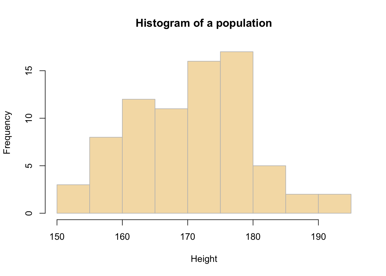

Figure 3.1: The distribution of the Height variable.

3.3.1 Take an initial sample

You can assess a sample of 10 observations (survey respondents) taken from the population at random using the sample function.

sample.10 <- sample(pop, 10)

From this the sample mean \(\bar{x}\) and sample standard deviation can be calculated:

mean(sample.10)

## [1] 168.4

sd(sample.10)

## [1] 6.328068

Note You will get a different values for these to the ones your friends get (and the ones created below), because you will have each extracted a different sample from the population - this is random sampling!

You should calculate the Standard Error (SE) of the sample mean and populate Table 3.1 after running the code below:

# sample standard deviation (as above)
sd(sample.10)
# sample SE
sd(sample.10)/sqrt(length(sample.10))

Table 3.1: Mean table.

Mean	Value
Population mean	171.4
Sample mean
SE mean

The Standard Error tells us how accurate the mean of any given sample from population, \(\bar{x}\), is likely to be when compared to the true population mean \(\mu\). High SEs indicate that it is more likely that the sample mean is an inaccurate representation of the true population mean.

In the case above, the sample standard error tells us that the sample may not be too representative of the population (unless we were very lucky in our sample).

3.3.2 Increasing the sample size

To see how using a larger sample improves the estimate, you will now repeat the previous example, generating a sample, determining the sample means and SEs, but using different sample sizes: 10, 20, 50, 70.

Task 1. Complete Table 3.2. You have already got the values for the sample of 10 created above, and you will need need to modify the code below, which is a summary of the code used thus far, for different sample sizes.

## Create a sample of the population
sample.10 <- sample(pop, 10)
## Mean and s.d.
mean(sample.10)
sd(sample.10)
## Standard Error
sd(sample.10)/sqrt(length(sample.10))

Table 3.2: Effects of increasing sample size.

Sample Size	10	20	50	70
Population mean	171.4	171.4	171.4	171.4
Sample Mean
Standard Error

The above should have given you the general idea that as sample size increases, the sample estimate of a population mean becomes more reliable. To show this clearly, the code below generates a trend line plot showing the impact of sample size on Standard Errors. As the sample gets larger the SE gets smaller as the sample more closely represents the true population.

# create a vector of sample sizes
X = seq(10, 70, 5)
# check the result
X

##  [1] 10 15 20 25 30 35 40 45 50 55 60 65 70

# create a vector of sample errors from these
# an empty vector to be populated in the for loop below
SE = vector()
# now loop though each value in X
for (i in X){
  # create a sample for the ith value in X
  # set the seed - see the Info box below
  set.seed(12)
  sample.i = sample(pop, i)
  # calculate the SE
  se.i = sd(sample.i)/sqrt(length(sample.i))
  # add to the SE vector
  SE = append(SE, se.i)
}
# check the result
SE

##  [1] 3.699586 2.614237 2.202691 2.094014 1.825524 1.761361 1.590520 1.435058
##  [9] 1.311411 1.245404 1.169452 1.124123 1.075558

You can then these plot these:

# plot the SEs
plot(x = X, y = SE,
     pch = 19, col = "dodgerblue",
     xlab = "Sample Size", ylab = "Standard Error", 
     main = "Impact of sample size on Standard Error")
lines(x = X, y = SE)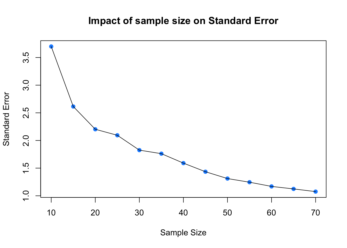

Figure 3.2: Sample size against SE.

So…as sample size increases, the sample estimate of a population mean becomes more reliable. However, you should note that this was based on one-off sample generation and looking at the SE. In the next section you will apply confidence intervals to the sample in order to assess the robustness of the sample.

3.3.3 Confidence Intervals

In this section you will calculate some confidence intervals to try to determine your sample reliability. We can use the qnorm function to calculate the errors around the sample mean under an assumption of a normal distribution of the population (hence the norm bit of qnorm):

# you have already created the sample with
# sample.10 <- sample(pop, 10)
m <- mean(sample.10)
std <- sd(sample.10)
n <- length(sample.10)
error <- qnorm(0.975)*std/sqrt(n)
lower.bound <- m-error
upper.bound <- m+error
# upper and lower bound
upper.bound

## [1] 172.3221

lower.bound

## [1] 164.4779

This is the 95% confidence interval (97.5% in two directions!)

Remembering that your values will be subtly different due to random sample, what this indicates is that we are 95% confident that the mean Height for the population is between 164.5 and 172.3.

BUT in this case, with a sample of 10, this is a very weak assertion with wide confidence intervals. Drawing a larger sample at random from our population will help to narrow these.

Task 3. You should modify the code above for the different sample sizes to complete Table 3.3, calculating the upper and lower bound for each sample size.

Table 3.3: Confidence Intervals for increased in sample size.

Sample Size	10	20	50	70
Population mean	171.4	171.4	171.4	171.4
Sample Mean
Sample Standard Deviation
Lower Bound
Upper Bound

What you should see is that as \(n\) gets larger, then the upper and lower bounds - the error bounds - get nearer to the sample mean. The critical thing here is to consider the errors in relation to the standard deviation.

As a final graphical trick, you can plot a fancy histogram using the errors / CIs you have calculated. In the plot in the figure below, the errors / CIs from the sample are shown in yellow, the standard deviations of the sample around the mean are in tomato and the main body of the plot is the whole population in grey - yes, tomato is a colour in R!

# first recreate the sample of 10 observations 
# to ensure reproducibility use set.seed()
set.seed(123)
sample.10 <- sample(pop, 10)
## Mean and s.d.
m <- mean(sample.10)
# and then calculate upper and lower CIs as before
std <- sd(sample.10)
n <- length(sample.10)
error <- qnorm(0.975)*std/sqrt(n)
lower.bound <- m-error
upper.bound <- m+error
## create a histogram object from the population to get the breaks out
h <- hist(pop, breaks  = 12, plot = F)
## create a vector of colours
col = rep("tomato", length(h$breaks))
## colour the histogram yellow between the Confidence Intervals
index <- h$breaks > lower.bound & h$breaks < upper.bound 
col[index] <- "#FFDC00" # this is a nice yellow!
## colour the histogram grey for values outside of Mean+St Dev and Mean-St Dev 
index <-  h$breaks < m-std | h$breaks > m+std
col[index] <- "grey"
## now plot
plot(h, col = col, 
    main = "Confidence intervals & St Dev, n = 10", 
    xlab = "Height", 
    border = NA)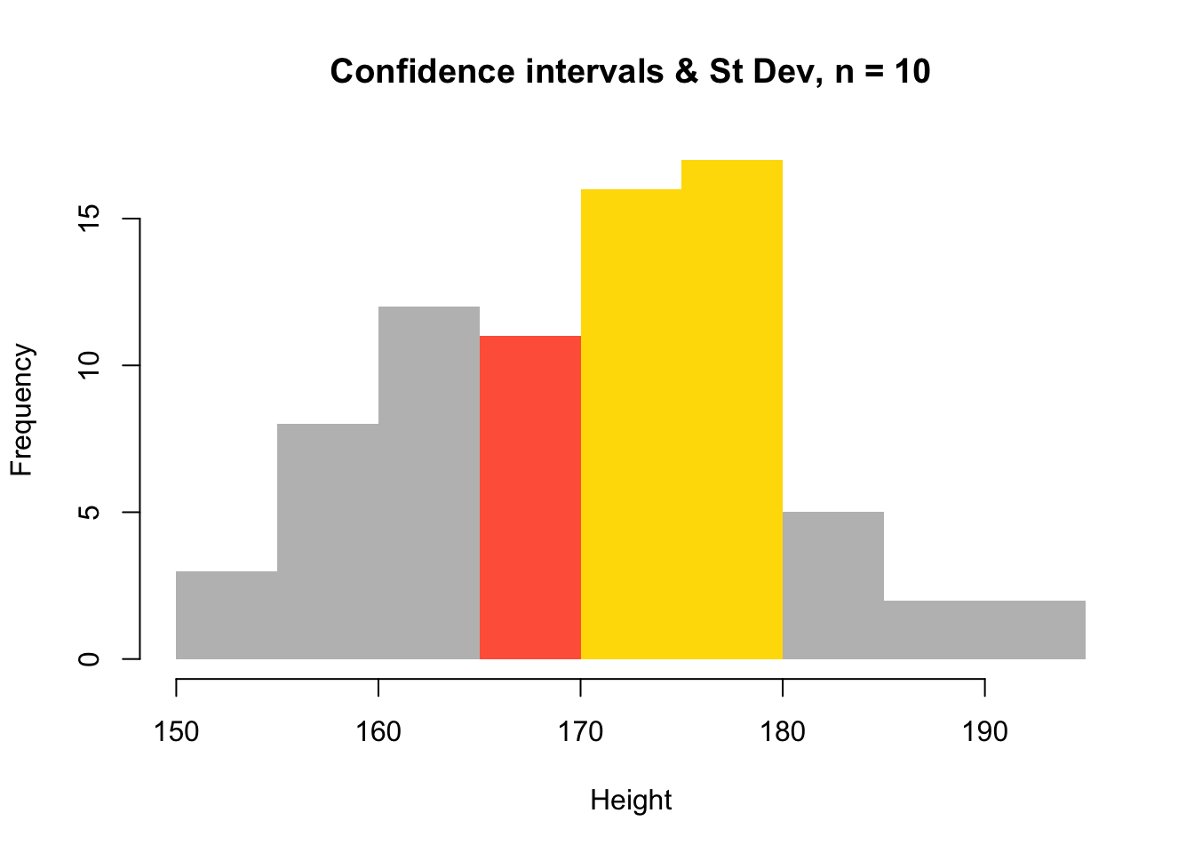

Figure 3.3: A histogram of the population with errors from a sample of 10 observations.

And compare this with the histogram when \(n\) = 60. First compute the sample and the associated statistics:

# to ensure reproducibility set.seed()
set.seed(121)
sample.60 <- sample(pop, 60)
m <- mean(sample.60)
std <- sd(sample.60)
n <- length(sample.60)
error <- qnorm(0.975)*std/sqrt(n)
lower.bound <- m-error
upper.bound <- m+error

Then plot using the same approach as above to generate the figure below:

## and plot again 
h <- hist(pop, breaks  = 12, plot = F)
col = rep("tomato", length(h$breaks))
index <- h$breaks > lower.bound & h$breaks < upper.bound 
col[index] <- "#FFDC00"
index <-  h$breaks < m-std | h$breaks > m+std
col[index] <- "grey"
plot(h, col = col, 
    main = "Confidence intervals & St Dev, n = 80", 
    xlab = "Height", 
    border = NA)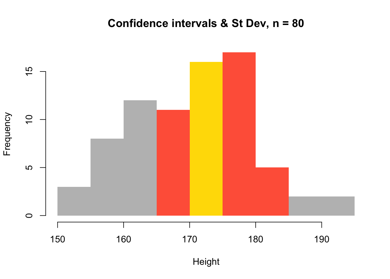

Figure 3.4: A histogram of the population with errors from a sample of 80 observations.

This shows a much narrower range than the first histogram which shows the errors and standard deviations from a sample where \(n\) = 10.

3.3.4 Summary

We often use a sample of the real population rather than the populations itself, for pragmatic reasons related to cost, time, availability of the population etc. However, one of the key issues is how representative is my sample of the true population. The Standard Error of the sample mean, provides a way of quantifying this. And by exploring the SEs of different sample sizes, we can see whether we have a large enough sample. However, any sample is by definition a random selection of observations, and samples of the same size may have very different properties. This is where confidence intervals come in. These use the idea of repeated sampling from the same population in order to get an estimation of the true population and to try to determine an optimal sample. It provides a level of confidence in our estimate of the population parameter (e.g. population mean) as derived from a sample.

3.4 Optional (ie not part of the portfolio)

Task 4.You have been playing with the data in df for a while now. Lets try and do something a bit more adventurous with it. Lets see if there is a difference in the number of piercings between survey respondents who went to State Secondary School up to 16 (StateSecondary16) and those that did not.

It is helpful to break any problem down to series of discrete stages. For this you will need to:

• create an index that selects the “Yes” responses to the StateSecondary16 variable.
• use that to subset the `Piercings variable for those respondents
• calculate the mean value of `Piercings for that group.
• finally do the same for the “No” responses to the StateSecondary16 variable.

The answer to this task is after the Resources section below.

Resources

Great summary of SE, samples and CIs: https://mgimond.github.io/Stats-in-R/CI.html

Standard Error:

• pages 92-93 in Harris (2016)
• https://www.greenbook.org/marketing-research/how-to-interpret-standard-deviation-and-standard-error-in-survey-research-03377
• https://s4be.cochrane.org/blog/2018/09/26/a-beginners-guide-to-standard-deviation-and-standard-error/

Optional Task Answer

Task 4. You have been playing with the data in df for a while now. Lets try and do something a bit more adventurous with it. Lets see if there is a difference in the number of piercings between survey respondents who went to State Secondary School up to 16 (StateSecondary16) and those that did not.

# select Yes responses to StateSecondary16 and assign to R object
x = df$StateSecondary16 == "Yes"
# use that to index df$Piercings
df$Piercings[x]
# calculate the mean 
mean(df$Piercings[x])

# select No responses to StateSecondary16 and assign to R object
x = df$StateSecondary16 == "No"
# use that to index df$Piercings
df$Piercings[x]
# calculate the mean 
mean(df$Piercings[x])

# All in one go
mean(df$Piercings[df$StateSecondary16 == "Yes"])
mean(df$Piercings[df$StateSecondary16 == "No"])