Chapter 1 Week 19: Getting Started in RStudio

About this book

This is an on-line book written to support the practicals for the GEOG1400 Digital Geographies module, delivered by Lex Comber of the School of Geography, from the University of Leeds. It is based on An Introduction to Spatial Analysis and Mapping (Brunsdon and Comber 2018 (link here) which provides a foundation for spatial data handling, GIS-related operations and spatial analysis in R.)

The chapters in this book contain an individual Practical with a discrete set of activities, and links to any required data and R packages. Each chapter is self contained and includes instructions for loading and data and packages as needed. An R script is provided for each session except this one. An R script is a text file with code, with the file extension .R

This chapter contains an Introduction to R that you should work through before Week 20. It demonstrates how to access R through RStudio on a university PC , via AppsAnywhere and undertakes some basic operations in R.

1.1 Starting RStudio

RStudio provides a convenient graphical interface to R. It can be accessed through AppsAnywhere. You need to log on to a University PC and in AppsAnywhere start R first before you launch RStudio.

The steps are:

Search for “Cran” and R is listed under Cran R 4.2.0 x64.
Click on Launch and then minimise the RGui window after it opens (NB this should be minimised and not closed).
Search for RStudio which is listed under Rstudio 2022.
Again click Launch and ignore any package or software updates.

You should have a new RStudio session.

This process is summarised in Figure 1.1.

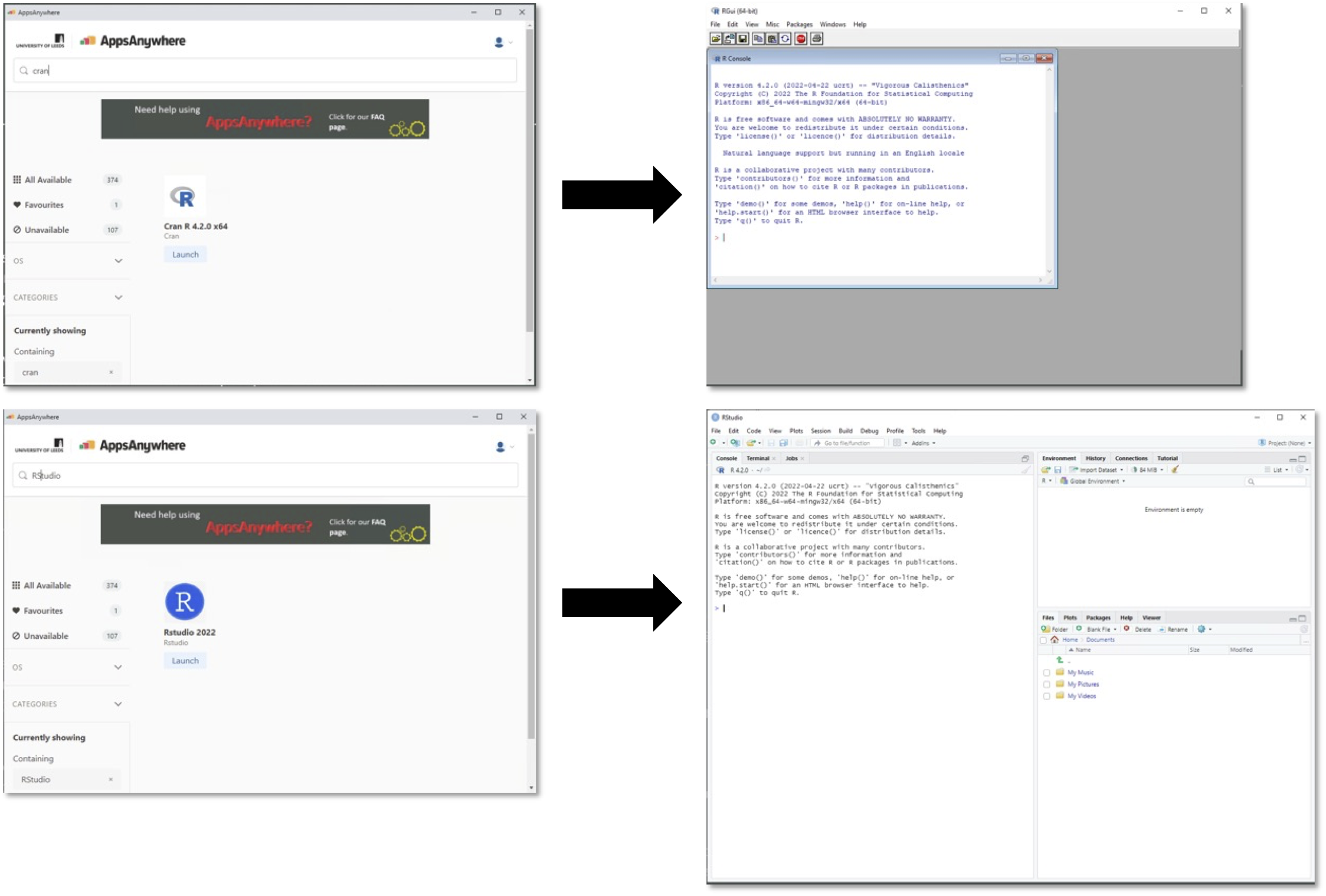
Figure 1.1: AppsAnywhere: launching R called Cran R (top), and RStudio (bottom).

1.2 File Managment

Now file management is really important. In Windows Explorer you should create a folder for your module practical work on your M-drive if you have not done so already. We suggested in the Week 14 practical that you create a folder called GEOG1400. In this you should create sub-folders for each practical session. You should already have some for Weeks 14 to 18 (Week19, Week20) etc.

For this session, create a sub-folder called Week19 in your GEOG1400 folder on your M-Drive. Recall that each week we have stressed the importance of this in the practicals:

Before you start installing software or downloading data, create a folder on your M-Drive (if working on a University networked machine) or locally if working on your own device – name this ‘GEOG1400’ and within this create a sub-folder – name this ‘Practical1’. This folder will store the data for this practical. For your assessed portfolio (in later weeks), you may be asked to submit some of this work, so it is best if you know where to find it. Take care to ensure you do not delete any work you do complete in the practical sessions. It is imperative that you practice good file management!

1.3 The RStudio interface

RStudio provides an interface to the different things that R can do via the 4 panes: the Console where code is entered (bottom left), a Source pane with R scripts (top left), the variables in the working Environment (top right), Files, Plots, Help etc (bottom right) - see the RStudio environment in Figure 1.2 below.

Figure 1.2: The RStudio environment.

In the figure above of the RStudio interface, a new script has been opened, a line of code had been written and then run in the console. The code assigns a value of 100 to x. The file has been saved into the current working environment. You are expected to define a similar set up for each practical as you work through the code. Note that in the script, anything that follows a # is a comment and ignored by R.

Users can set up their personal preferences for how they like their RStudio interface. Similar to straight R, there are very few pull-down menus in R, and therefore you will type lines of code into your script and run these in what is termed a command line interface (the console). Like all command line interfaces, the learning curve is steep but the interaction with the software is more detailed which allows greater flexibility and precision in the specification of commands.

Beyond this there are further choices to be made. Commands can be entered in two forms: directly into the R console window or as a series of commands into a script window. We strongly advise that all code should be written in a script - (a .R file) and then run from the script. - To run code in a script, place the cursor on the line of code and then run by pressing the ‘Run’ icon at the top left of the script pane, or by pressing Ctrl Enter (PC) (or Cmd Enter on a Mac).

1.4 Ways of working

The first set of consideration relate to how you should work in R/RStudio. The key things to remember are:

R is a learning curve if you have never done anything like this before. It can be scary. It can be intimidating. But once you have a bit of familiarity with how things work, it is incredibly powerful.
You will be working from practical worksheets which will have all the code you need. Your job is to try to understand what the code is doing and not to remember the code. Comments in your code really help.
To help you do this, the very strong suggestion is use the R scripts that are provided, and that you add your own comments to help you understand what is going on when you return to them. Comments are prefaced by a hash (#) that is ignored by R. Then you can save your code (with comments), run it and return to it later and modify at your leisure.

The module places a strong emphasis placed on learning by doing, which means that you encouraged to unpick the code that you are given, adapt it and play with it. It is not about remembering or being able to recall each function used but about understanding what is being done. If you can remember what you did previously (i.e. the operations you undertook) and understand what you did, you will be able to return to your code the next time you want to do something similar. To help you with this you should:

Always run your code from an R script… always! These are provided for each practical;
Annotate you scripts with comments. These are prefixed by a hash (#) in the code;
Save your R script to your folder;

To summarise…

You should always use a script (a text file containing code) for your code which can be saved and then re-run at a later date.
You can write your own code into a script, copy and paste code into it or use an existing script (for example as provided for each of the R/RStudio practicals in this module).
To open a new R script go to File > New File > R Script to open a new R file, and save it with a sensible name.
To load an existing script file go to File > Open File and then navigate to your file. Or, if you have recently opened the file, go to File > Recent Files >.
It is good practice to set the working directory at the beginning of your R session. This can be done via the menu in RStudio Session > Set Working Directory > …. This points the R session to the folder you choose and will ensure that any files you wish to read, write or save are placed in this directory.
To run code in a script, place the cursor on the line of code and then run by pressing the ‘Run’ icon at the top left of the script pane, or by pressing Ctrl Enter (PC) or Cmd Enter (Mac).

1.5 Your first R code

In this section you will undertake a few generic operations. You will:

undertake assignment: the allocation of values to an R object.
use assignment to create a vector of elements and a matrix of elements.
undertake operations on R objects.
apply some functions to R objects (functions nearly always return a value).
access some of R in-built data to examine a data table (or data.frame which is like an Excel spreadsheet).
do some basic plotting, including scatter plots and histograms.
create data summaries.

On the way you will also be introduced to indexing.

First, you should create a new R script (see above) and save it as week19.R in the working directory you are using for this practical. This should be the Week19 sub-directory you created in the GEOG1400 folder. Note that you should create a separate folder for each week’s practical.

1.5.1 Assignment

The command line prompt in the Console window, the >, is an invitation to start typing in your commands.

Write the following into your script: 2+2 and run it. Recall that code is run done by either by pressing the Run icon at the top left of the script pane, or by pressing Ctrl Enter (PC) or Cmd Enter (Mac).

2+2

## [1] 4

Here the result is 4. The [1] that precedes the output it formally indicates, first requested element will follow. In this case there is just one element. The > indicates that R is ready for another command.

Now type the following in to your script and run it:

y <- 2+2
y

## [1] 4

Here the value of the 2+2 has been assigned to y. The syntax y <- 2+2 can be read as y gets 2+2. When y is invoked its value is returned (4).

For the purposes of this module, in R the equals sign (=) is the same as <-, a left diamond bracket < followed by a minus sign -. This too is interpreted by R as is assigned to or gets when the code is read right to left.

Now copy and paste the following into your R script and run both lines:

x <- matrix(c(1,2,3,4,5,6,7,8), nrow = 4)
y = matrix(1:8, nrow = 4, byrow = T)

You should see the x appear with the y in the Environment pane. y has now been overwritten with a new assignment. If you click on the icon next to them, you will get a ‘spreadsheet’ view of the data you have created.

Of course you can also enter the following in the console and see what is returned:

x
y

Note In the code snippets above you have used parentheses - round brackets. Different kinds of brackets are used in different ways in R. Parentheses are used with functions, and contain the arguments that are passed to the function, separated by commas (,).

In this case the functions are c() and matrix(). The function c() combines or concatenates elements into a vector, and matrix() creates a matrix of elements in a tabular format.

In the line of code x = matrix(c(1,2,3,4,5,6,7,8), nrow = 4), the arguments passed to the matrix() function are the vector of values c(1,2,3,4,5,6,7,8) and nrow = 4. Other kinds of brackets are used in different ways as you will see later.

One final thing to note is that the matrix is y is has the numbers 1 to 8, but this is specified by 1:8. Try entering 3:65, 19:11, and 1.5:5 to see how the colon (:) works in this context.

1.5.2 Operations

Now you can undertake operations on R objects and apply functions to them. Write the following code into your script and then run it:

# x is a matrix
x
# multiplication
x*2
# sum of x
sum(x)
# mean of x
mean(x)

Operations can be undertaken directly using mathematical notation like * for multiplication or using functions like max to find the maximum value in an R object.

1.5.3 Functions

Functions are always followed by parenthesis (round brackets) ( ). These are different from square and curly brackets [ ] and { }. Functions always return something, a result if you like, and have the generic form:

# don't run this or write this into your script!
result = function(value or R object, other parameters)

Do not run or enter this code in your script - it is an example!

1.5.4 Data Tables

Here we will load a data table in data.frame (like a spreadsheet) in R/RStudio. R has number of in-built datasets that we can use the code below loads one of these:

data(mtcars)
class(mtcars)

## [1] "data.frame"

Have a look at what is loaded by listing the objects in the current R session

ls()

## [1] "mtcars" "x"      "y"

You should see the mtcars object. You can examine this data in a number of ways

# the structure of mtcars
str(mtcars)

## 'data.frame':    32 obs. of  11 variables:
##  $ mpg : num  21 21 22.8 21.4 18.7 18.1 14.3 24.4 22.8 19.2 ...
##  $ cyl : num  6 6 4 6 8 6 8 4 4 6 ...
##  $ disp: num  160 160 108 258 360 ...
##  $ hp  : num  110 110 93 110 175 105 245 62 95 123 ...
##  $ drat: num  3.9 3.9 3.85 3.08 3.15 2.76 3.21 3.69 3.92 3.92 ...
##  $ wt  : num  2.62 2.88 2.32 3.21 3.44 ...
##  $ qsec: num  16.5 17 18.6 19.4 17 ...
##  $ vs  : num  0 0 1 1 0 1 0 1 1 1 ...
##  $ am  : num  1 1 1 0 0 0 0 0 0 0 ...
##  $ gear: num  4 4 4 3 3 3 3 4 4 4 ...
##  $ carb: num  4 4 1 1 2 1 4 2 2 4 ...

# the first six rows (or head) of mtcars
head(mtcars)

##                    mpg cyl disp  hp drat    wt  qsec vs am gear carb
## Mazda RX4         21.0   6  160 110 3.90 2.620 16.46  0  1    4    4
## Mazda RX4 Wag     21.0   6  160 110 3.90 2.875 17.02  0  1    4    4
## Datsun 710        22.8   4  108  93 3.85 2.320 18.61  1  1    4    1
## Hornet 4 Drive    21.4   6  258 110 3.08 3.215 19.44  1  0    3    1
## Hornet Sportabout 18.7   8  360 175 3.15 3.440 17.02  0  0    3    2
## Valiant           18.1   6  225 105 2.76 3.460 20.22  1  0    3    1

The mtcars object is a data.frame, a kind of data table, and it has a number of attributes which are all numeric. The code below prints it all out to the console:

mtcars

Data frames are ‘flat’ in that they typically have a rectangular layout like a spreadsheet, with rows typically relating to observations (individuals, areas, people, houses, etc) and columns relating to their properties or attributes (height, age, etc). The columns in data frames can be of different types: vectors of numbers, factors (classes) or text strings. In matrices all of the columns have to be off the same type. Data frames are central to what we will do in R.

1.5.5 Plotting the data: ‘Hello World!’

The code below creates a plot of 2 variables counts in the data: mpg and disp.

plot(disp ~ mpg,  data = mtcars, pch=16)

The option pch=16 sets the plotting character to a solid black dot. More plot characters are available - examine the help for points() to see these:

?points

This plot can be improved greatly. We can specify more informative axis labels, change size of the text and of the plotting symbol, and so on.

We can also specify the same plot by passing named variables to the plot function directly as well as other parameters, as in the figure. Notice how the syntax for this is different to the plot function above, and the different parameters that are passed to the plot() function:

plot(x = mtcars$mpg, y = mtcars$disp,   pch = 1, col = "dodgerblue", 
     cex = 1.5, xlab = "Miles per Gallon", ylab = "Displacement", 
     main = "Hello World!")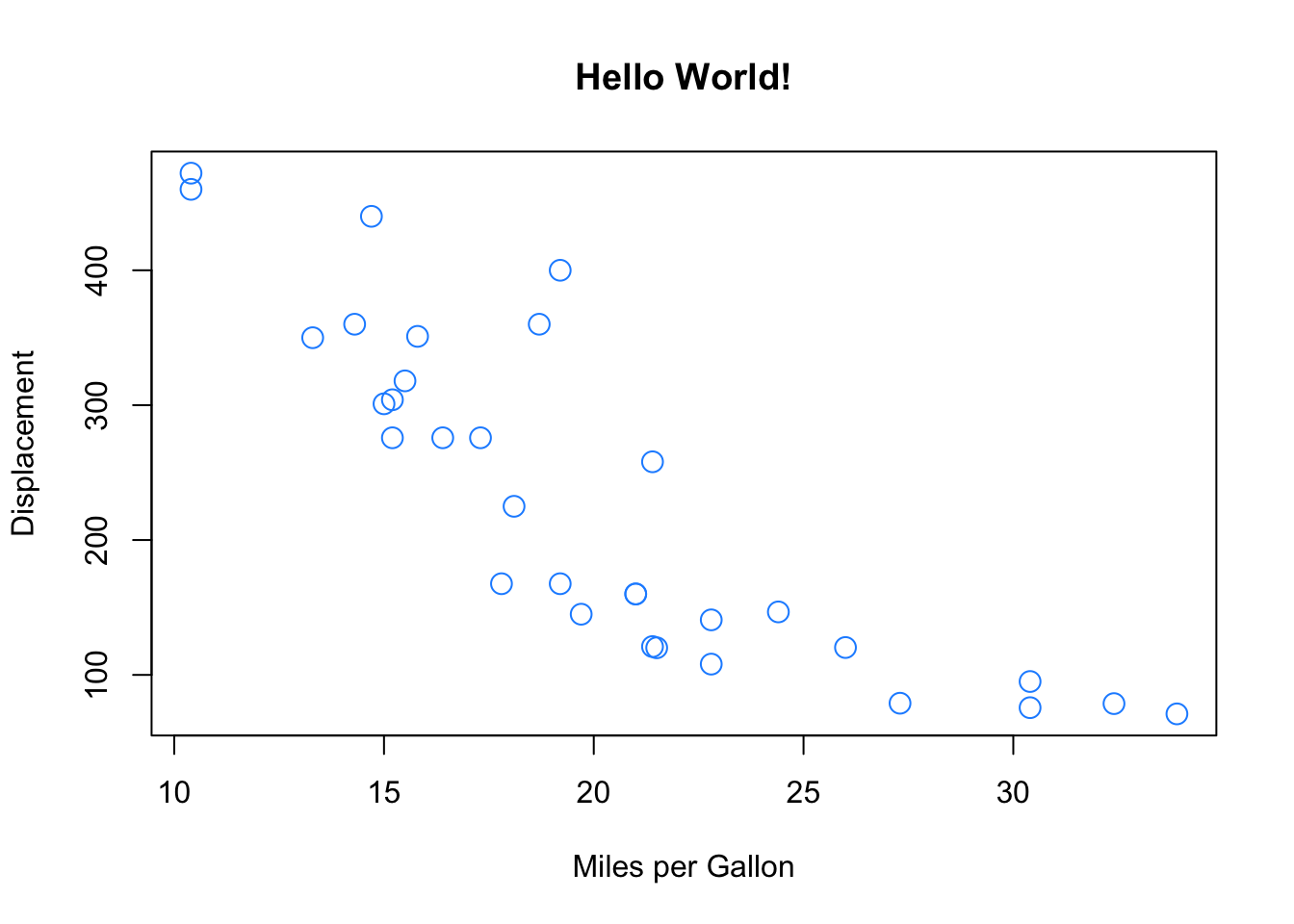

Figure 1.3: A scatter plot.

Notice how the dollar sign ($) is used to access variables in the mtcars data table compared to the first plot command, which specified data = mtcars.

1.5.6 Data summaries and indexing

We may for example require information on variables in mtcars. The summary function is very useful:

summary(mtcars)

##       mpg             cyl             disp             hp       
##  Min.   :10.40   Min.   :4.000   Min.   : 71.1   Min.   : 52.0  
##  1st Qu.:15.43   1st Qu.:4.000   1st Qu.:120.8   1st Qu.: 96.5  
##  Median :19.20   Median :6.000   Median :196.3   Median :123.0  
##  Mean   :20.09   Mean   :6.188   Mean   :230.7   Mean   :146.7  
##  3rd Qu.:22.80   3rd Qu.:8.000   3rd Qu.:326.0   3rd Qu.:180.0  
##  Max.   :33.90   Max.   :8.000   Max.   :472.0   Max.   :335.0  
##       drat             wt             qsec             vs        
##  Min.   :2.760   Min.   :1.513   Min.   :14.50   Min.   :0.0000  
##  1st Qu.:3.080   1st Qu.:2.581   1st Qu.:16.89   1st Qu.:0.0000  
##  Median :3.695   Median :3.325   Median :17.71   Median :0.0000  
##  Mean   :3.597   Mean   :3.217   Mean   :17.85   Mean   :0.4375  
##  3rd Qu.:3.920   3rd Qu.:3.610   3rd Qu.:18.90   3rd Qu.:1.0000  
##  Max.   :4.930   Max.   :5.424   Max.   :22.90   Max.   :1.0000  
##        am              gear            carb      
##  Min.   :0.0000   Min.   :3.000   Min.   :1.000  
##  1st Qu.:0.0000   1st Qu.:3.000   1st Qu.:2.000  
##  Median :0.0000   Median :4.000   Median :2.000  
##  Mean   :0.4062   Mean   :3.688   Mean   :2.812  
##  3rd Qu.:1.0000   3rd Qu.:4.000   3rd Qu.:4.000  
##  Max.   :1.0000   Max.   :5.000   Max.   :8.000

This shows different summaries of the individual attributes in mtcars.

The main R graphics function is plot(). In addition to plot() there are functions for adding points and lines to existing graphs, for placing text at specified positions, for specifying tick marks and tick labels, for labelling axes, and so on.

There are various other alternative helpful forms of graphical summary. A helpful graphical summary for the mtcars data frame is the scatterplot matrix, shown in Figure 1.4.

# return the names of the mtcars variables
names(mtcars)

##  [1] "mpg"  "cyl"  "disp" "hp"   "drat" "wt"   "qsec" "vs"   "am"   "gear"
## [11] "carb"

# return the 3rd to 7th names
names(mtcars)[c(3:7)]

## [1] "disp" "hp"   "drat" "wt"   "qsec"

# check what this does
c(3:7)

## [1] 3 4 5 6 7

# plot the 3rd to 7th variables in mtcars
plot(mtcars[, c(3:7)], cex = 0.5, 
     col = "red", upper.panel=panel.smooth)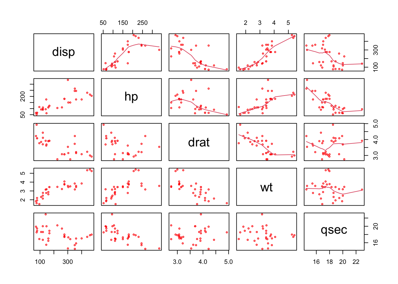

Figure 1.4: Multiple scatterplots.

The results show the correlations between the variables in the mtcars data frame, and the trend of their relationship is included with the upper.panel=panel.smooth parameter passed to plot.

There are number of things to notice here (as well as the figure). In particular note the use of the vector c(2:7) to subset the columns of mtcars:

In the second line, this is was used to subset the vector of column names created by names(mtcars).
In the third line, it was printed out. Notice how 3:7 printed out all the number between 3 and 7 - very useful.
For the plot, the vector was passed to the second argument, after the comma, in the square brackets [,] to indicate which columns were to be plotted.

The referencing in this way (or indexing) is very important: the individual rows and columns of 2 dimensional data structures like data frames, matrices, tibbles etc can be accessed by passing references to them in the square brackets.

# 1st row
mtcars[1,]
# 3rd column
mtcars[,3]
# a selection of rows
mtcars[c(3:5,8),]

Such indexing could of course have been assigned to a R object and used to do the subsetting:

x = c(3:7)
names(mtcars)[x]
plot(mtcars[,x], cex = 0.5, col = "red")

Thus indexing allows specific rows and columns to be extracted from the data as required.

Note You have encountered a second type of brackets, square brackets [ ]. These are used to reference or index positions in a vector or a data table.

Consider the object x above. It contains a vector of values, 3,4,5,6,7. Entering x[1] would extract the first element of x, in this case 3. Similarly x[4] would return the 4th element and x[c(1,4)] would return the 1st and 4th elements of x.

However, in the examples above that index the 2-dimensional mtcars object, the square brackets are used to index row and column positions. The syntax for this is [rows, columns]. We will be using such indexing throughout this module.

1.6 Some Tasks

Recall that a data.frame is a rectangular array of columns of data. Here you will create a data frame of two columns containing numeric values. The following data gives the distance that an elastic band moves when released for each amount it is stretched over the end of a ruler:

elasticband <- data.frame(stretch=c(46,54,48,50,44,42,52),
                          distance=c(148,182,173,166,109,141,166))
# have a look
elasticband

##   stretch distance
## 1      46      148
## 2      54      182
## 3      48      173
## 4      50      166
## 5      44      109
## 6      42      141
## 7      52      166

The function data.frame() can be used to input these (or other) data directly into data.frame objects.

Task 1 Plot distance against stretch from the elasticband data frame.

Task 2 Use the hist() command to plot a histogram of the mpg values in the mtcars data frame. Hints: a) think about how the Hello World plot was parameterised and the fact that histograms are constructed from a single variable, and b) examine the help for hist by entering ?hist at the console.

Task 3 Repeat 2 after taking logarithms of disp cover using the log() function - i.e. do a histogram of `log(mtcars$mpg)

Answers to the tasks are at the end of the practical.

1.7 Packages

The base installation of R includes many functions and commands. However, more often we are interested in using some particular functionality, encoded into packages contributed by the R developer community. Installing packages for the first time can be done at the command line in the R console using the install.packages command as in the example below to install the tmap library or via the RStudio menu via Tools > Install Packages.

When you install these packages it is strongly suggested you also install the dependencies. These are other packages that are required by the package that is being installed. This can be done by selecting check the box in the menu or including dep=TRUE in the command line as below (don’t run this yet!):

# don't run this!
install.packages("tidyverse", dep = TRUE)

You may have to set a mirror site from which the packages will be downloaded to your computer. Generally you should pick one that is nearby to you.

Further descriptions of packages, their installation and their data structures will be given as needed in the practicals. There are literally 1000s of packages that have been contributed to the R project by various researchers and organisations. These can be located by name at http://cran.r-project.org/web/packages/available_packages_by_name.html if you know the package you wish to use. It is also possible to search the CRAN website to find packages to perform particular tasks at http://www.r-project.org/search.html. Additionally many packages include user guides and vignettes as well as a PDF document describing the package and listed at the top of the index page of the help files for the package.

As well as tidyverse you should install the sf package and dependencies. So we have 2 packages to install:

sf for spatial data and spatial objects
tidyverse for lots of lovely data science things - see https://www.tidyverse.org

You could do this in one go and this will take a bit of time:

install.packages(c("sf", "tidyverse"), dep = TRUE)

Remember: you will only have to install a package once!! So when the above code has run in your script you should comment it out. For example you might want to include something like the below in your R script.

# packages only need to be loaded once
# install.packages(c("sf", "tidyverse"), dep = TRUE)

Once the package has been installed on your computer then the package can be called using the library() function into each of your R sessions as below.

library(sf)

Finally you can save your R script, week19.R it should look something like the below:

# Week 19 script

# assignment
2+2 
y <- 2+2
# have a look at y
y

# make matrices
x <- matrix(c(1,2,3,4,5,6,7,8), nrow = 4)
y = matrix(1:8, nrow = 4, byrow = T)
# have a look at these
x
y
# x is a matrix
x

# operations
# multiplication
x*2
# sum of x
sum(x)
# mean of x
mean(x)

# load some inbuilt data
data(mtcars)
# inspect the class of mtcars
class(mtcars)

# list all objects in my working environment
ls()

# the structure of mtcars
str(mtcars)
# the first six rows (or head) of mtcars
head(mtcars)

# print out all of mtcars
mtcars

# plot mpg against disp
plot(disp ~ mpg,  data = mtcars, pch=16)

# the help for points
?points

# an enhanced plot using a different notation
plot(x = mtcars$mpg, y = mtcars$disp,   pch = 1, col = "dodgerblue", 
     cex = 1.5, xlab = "Miles per Gallon", ylab = "Displacement", main = "Hello World!")

# summaries fo all the variables in mtcars
summary(mtcars)

# return the names of the mtcars variables
names(mtcars)
# return the 3rd to 7th names
names(mtcars)[c(3:7)]
# check what this does
c(3:7)
# plot the 3rd to 7th variables in mtcars
plot(mtcars[, c(3:7)], cex = 0.5, 
     col = "red", upper.panel=panel.smooth)

# 1st row
mtcars[1,]
# 3rd column
mtcars[,3]
# a selection of rows
mtcars[c(3:5,8),]

# assign 3:7 to x
x = c(3:7)
# get the 3rd to 7th names in mtcars using x
names(mtcars)[x]
# recreate the plot 
plot(mtcars[,x], cex = 0.5, col = "red")

# some tasks
elasticband <- data.frame(stretch=c(46,54,48,50,44,42,52),
                          distance=c(148,182,173,166,109,141,166))
# have a look
elasticband

# don't run this!
# install.packages("tidyverse", dep = TRUE)

# packages only need to be loaded once
# install the packages in one go and THEN comment out
# install.packages(c("sf", "tidyverse"), dep = TRUE)

# load a package 
library(sf)

## Answers to tasks
# Task 1
plot(stretch~distance, data = elasticband)
# or
plot(elasticband$stretch, elasticband$distance)

# Task 2
hist(mtcars$mpg)

hist(mtcars$mpg, xlab='Miles per Gallon',
     main='Histogram of MPG',
     breaks = 15,
     col = 'DarkRed')

hist(mtcars$mpg, prob = T,
     xlab='Miles per Gallon',
     main='Histogram of MPG',
     breaks = 15,
     col = 'DarkRed',
     border = "#FFFFBF")
# add the probability density trend
lines(density(mtcars$mpg, na.rm=T),col='salmon',lwd=2)
# show the frequencies at the bottom - like a rug!
rug(mtcars$mpg)

# Task 3
hist(log(mtcars$mpg))

1.8 Summary

The aim of this session has been to familiarise you with the R environment if you have not used R before. If you have but not for a while, then hopefully this has acted as a refresher. Some key things to take away are:

R is a learning curve, and like driving the more your practice the better you become.
Your job is to try to understand what the code is doing and not to remember the code.
To help with this, you should add your own comments to the script to help you understand what is going on when you return to them. Comments are prefaced by a hash (#) that is ignored by R.
Always set your working directory to the sub-folder containing your R script.
Always run your code from an R script… always!

The reading for this week is Harris (2016) Chapter 12 up to page 282. You do not have to install any packages (Section 12.2), packages will be introduced in Week 20, but you should try some of the code. Go through the illustrations in Section 12.3 (The Basics of R, starting p253), entering commands with your comments in the script (prep.R) that you created above.

Optionally you could also briefly read or skim Section 12.3 - the sections are mis-numbered (A Geographical Introduction to R, starting p261), as we will cover these in more detail in subsequent weeks and modules. Go through the Section 12.3 (A Little More about the Workings of R, starting on p268), again entering commands in the script that you created above. Don’t worry about regression (top of p273) we will cover this later, but pay attention to Data Frames (p274), Referencing rows and columns (p275) and Subsetting (p279). Stop at Reading Data (p282).

Other good on-line get started in R guides include:

The Owen guide (only up to page 28) : https://cran.r-project.org/doc/contrib/Owen-TheRGuide.pdf
An Introduction to R - https://cran.r-project.org/doc/contrib/Lam-IntroductionToR_LHL.pdf
R for beginners https://cran.r-project.org/doc/contrib/Paradis-rdebuts_en.pdf

And of course there are my own offerings:

Comber and Brunsdon (2021) provide a through grounding of the topics covered in this module. Chapter 1 will support this introduction, and the code for each chapter is here: https://study.sagepub.com/comber/student-resources/code-library

Brunsdon and Comber (2018) provide a comprehensive introduction to R and spatial data: see https://uk.sagepub.com/en-gb/eur/an-introduction-to-r-for-spatial-analysis-and-mapping/book258267.

Answers to Tasks

Task 1 Plot distance against stretch from the elasticband data frame.

plot(stretch~distance, data = elasticband)
# or
plot(elasticband$stretch, elasticband$distance)

Task 2 Use the hist() command to plot a histogram of the mpg values in the mtcars data frame (hints: a) think about how the Hello World plot was parameterised and the fact that histograms are constructed from a single variable, and b) examine the help for hist by entering ?hist at the console)

hist(mtcars$mpg)

Of course, some refinement is possible.

hist(mtcars$mpg, xlab='Miles per Gallon', 
     main='Histogram of MPG', 
     breaks = 15,
     col = 'DarkRed')

The code below plots a probability density of the same data. Essentially what this does is normalize the histogram total are to 1.

hist(mtcars$mpg, prob = T, 
     xlab='Miles per Gallon', 
     main='Histogram of MPG', 
     breaks = 15,
     col = 'DarkRed',
     border = "#FFFFBF")
# add the probability density trend
lines(density(mtcars$mpg, na.rm=T),col='salmon',lwd=2)
# show the frequencies at the bottom - like a rug!
rug(mtcars$mpg)

Task 3 Repeat 2 after taking logarithms of mpg cover using the log() function:

hist(log(mtcars$mpg))

Appendix: Local installations of RStudio

R and RStudio can be downloaded from the CRAN website and installed your own computer - see below for details. A key point is that you should install R before you install RStudio.

The simplest way to get R installed on your computer is to go the download pages on the R website - a quick search for `download R’ should take you there, but if not you could try:

Windows: https://cran.r-project.org/bin/windows/base/
Mac: https://cran.r-project.org/bin/macosx/
Linux: http://cran.r-project.org/bin/linux/

The Windows and Mac version come with installer packages and are easy to install whilst the Linux binaries require use of a command terminal.

RStudio can be downloaded from https://www.rstudio.com/products/rstudio/download/ and the free version of RStudio Desktop is more than sufficient for this module and all the other things you will to do at degree level.

References

Brunsdon, Chris, and Lex Comber. 2018. An Introduction to r for Spatial Analysis and Mapping (2e). Sage.

Comber, Lex, and Chris Brunsdon. 2021. Geographical Data Science and Spatial Data Analysis: An Introduction in r. Sage.

Harris, Richard. 2016. Quantitative Geography: The Basics. Sage.

GEOG1400 Digital Geographies - RStudio Practicals