Chapter 3 Additional - Determining model form
3.1 Overview
In this session you will:
- Reflect on the assumptions associated with different model forms or specifications
- Evaluate different STVC models relating to how space and time interact using BIC
- Undertake Bayesian Model Averaging to combine the highly probable models
You should make sure the data and required packages are loaded as in Session 1
3.2 What model form?
How should you specify your STVC model?
The STCV model specified earlier included space and time in a single splines for each the covariates. This is to assume that that spatial and temporal processes do interact and that the temporal trends in predictor-target variable relationships will vary with location. But is this assumption correct? If you have a specific a hypothesis that you are testing or working under a particular theory related to how space and time interact in the process you are examining, then you can simply specify how the covariates interact with target variable. However, more commonly we are seeking inference (understanding) about how processes interact in space and time.
In this section, these are explored using a data driven (rather than theoretical) approach. In this section you will create different models, with different assumptions, and evaluate them to determine which one or set fo models is / are the most probable.
Multiple models can be created to explore all possible combinations of interaction and then to select the best model, through a probability based measure like BIC (see Comber et al. (submitted) for a full treatment of this). There are a total 6 possible way that each covariate could be specified in the model:
- It is omitted.
- It is included as a parametric response with no spline.
- It is included in a spline with location.
- It is included a spline with time.
- It is included in a single spline with location and time.
- It is included in 2 separate splines with location and time.
The intercept can be treated similarly, but without it being absent (i.e. 5 options).
To investigate model form, a series of models were specified, with each combination of the 6 permutations for each covariate, plus 5 states for the intercept. The best model(s) can be determined by quantifying the likelihood (probability) of each of model being the correct model. This can be approximated using the Bayesian Information Criterion (BIC) (Schwarz 1978) as described in full in Comber et al. (submitted), and if the probabilities for multiple models are high, then the models can be combined using a Bayesian Model Averaging (BMA) approach. BMA is described in the context of spatial modelling in Fragoso, Bertoli, and Louzada (2018) and summarised in Brunsdon, Harris, and Comber (2023), but in brief, if a number of competing models exist with at least one quantity of interest that all have in common, and the likelihoods of each of them being the correct model is known (e.g. from BIC ), then a posterior distribution of the quantity of interest can be obtained by averaging them using the likelihoods as weights. In this way it allows competing models, treating space and time in different ways, to be combined.
3.3 Create multiple models
To undertake this, the code with below first defines a grid of numbers for each covariate. This is passed to a function to create the formula specifying different models, with different terms and smooths, which in turn is passed to the gam function.
# define intercept term
produc <- produc |> mutate(one = 1)
# define grid of combinations (nrow = 180)
terms_gr = expand.grid(intcp = 1:5, unemp = 1:6, pubC = 1:6)
# examine a random slice
terms_gr |> slice_sample(n = 6)
## intcp unemp pubC
## 1 1 2 4
## 2 5 5 2
## 3 4 1 2
## 4 1 4 6
## 5 4 3 2
## 6 1 5 3A function is defined to create the equations: here this is bespoke to the covariate names and number:
library(glue)
library(purrr)
# define a function to make the equations
makeform_prod <- function(intcp, unemp, pubC, bs='gp') {
  #coords <-    c("X,Y",    "X2,Y2")[coords]
  intx <- c("",
            glue("+s(year,bs='{bs}',by=one)"),
            glue("+s(X,Y,bs='{bs}',by=one)"),
            glue("+s(X,Y,bs='{bs}',by=one) + s(year,bs='{bs}',by=one)"),
            glue("+s(X,Y,year,bs='{bs}',by=one)"))[intcp]
  unempx <- c("",
              "+ unemp",
              glue("+s(year,bs='{bs}',by=unemp)"),
              glue("+s(X,Y,bs='{bs}',by=unemp)"),
              glue("+s(X,Y,bs='{bs}',by=unemp) + s(year,bs='{bs}',by=unemp)"),
              glue("+s(X,Y,year,bs='{bs}',by=unemp)"))[unemp]
  pubCx <- c("",
             "+ pubC",
             glue("+s(year,bs='{bs}',by=pubC)"),
             glue("+s(X,Y,bs='{bs}',by=pubC)"),
             glue("+s(X,Y,bs='{bs}',by=pubC) + s(year,bs='{bs}',by=pubC)"),
             glue("+s(X,Y,year,bs='{bs}',by=pubC)"))[pubC]
  return(formula(glue("privC~one-1{unempx}{intx}{pubCx}")))
}
To see how this works, the code below passes some numbers to it
## privC ~ one - 1 + unemp + s(X, Y, year, bs = "gp", by = one) +
##     s(X, Y, bs = "gp", by = pubC)
## <environment: 0x7f9c0d0c8588>
Next a function to undertake the analysis and record the BIC, the indices and the formula is defined and tested:
do_gam = function(i){
    f <- makeform_prod(intcp = terms_gr$intcp[i],
                     unemp = terms_gr$unemp[i],
                     pubC = terms_gr$pubC[i],
                     bs='gp')
    # m = gam(f,data=df_lg_sy_z)
    m = gam(f,data=produc)
    bic = BIC(m)
    index = data.frame(intcp = terms_gr$intcp[i],
                       unemp = terms_gr$unemp[i],
                       pubC = terms_gr$pubC[i])
    f = paste0('privC~', as.character(f)[3] )
    return(data.frame(index, bic, f))
    #return(bic)
}Finally, this can be put in a loop to evaluate all of the potential space-time models:
t1 = Sys.time()
res_gam <- NULL
for(i in 1:nrow(terms_gr)) {
  res.i = do_gam(i)
  res_gam = rbind(res_gam, res.i)
}
Sys.time() - t1 # ~2 minutes
## Time difference of 1.631957 minsFor more complex problems, you could parallelise the loop if you have a large multivariate analyses:
# set up the parallelisation
library(doParallel)
cl <- makeCluster(detectCores()-1)
registerDoParallel(cl)
# do the parallel loop
t1 = Sys.time()
res_gam <-
  foreach(i = 1:nrow(terms_gr_prod),
          .combine = 'rbind',
          .packages = c("glue", "mgcv", "purrr")) %dopar% {
            do_gam_prod(i)
            }
Sys.time() - t1 # 20 seconds
# release the cores
stopCluster(cl)
3.4 Model probabilities
Having generated multiple models and recorded the BIC values for them, it is possible to generate probabilities for each model and evaluate them. The logics and supporting equations for this evaluations of each mode are detailed in Comber et al. (submitted). The results need to be sorted, the best 10 models identified, their structures extracted and then their relative probabilities calculated:
# sort the results
mod_comp <- tibble(
    res_gam) |>
    rename(BIC = bic) |>
    arrange(BIC)
# transpose the indices to to model terms
# rank and return the top 10 results
int_terms <- \(x) c("Fixed","s_T", "s_S", "s_T + S_S", "s_ST")[x]
var_terms <- \(x) c("---", "Fixed","s_T", "s_S", "s_T + s_S", "s_ST")[x]
mod_comp_tab <-
  mod_comp |>
  slice_head(n = 10) |>
  mutate(across(unemp:pubC,var_terms)) |>
  mutate(intcp = int_terms(intcp)) |>
  rename(`Intercept` = intcp,
         `Unemployment.` = unemp,
         `Public Captial` = pubC) |>
  mutate(Rank = 1:n()) |>
  relocate(Rank) |>
  select(-f)
# determine the relative probabilities
# ie relative to the top ranked model
p1_vec = NULL
for(i in 2:10) {
  p1 = exp(-(mod_comp_tab$BIC[i]-mod_comp_tab$BIC[1])/2)
  p1 = p1/(1+p1)
  p1_vec = c(p1_vec, p1)
}
mod_comp_tab$`Pr(M)` = c("--", paste0(format(round(p1_vec*100, digits=1), nsmall = 1), "%"))The results are shown in Table 3.1 and suggest that nine of the models are highly probable, each with probabilities of better than the best ranked model of >10%. These are candidates for Bayesian Model Averaging. The are some commonalities in the specification of the 4 models:
- It does not matter whether the Intercept varies over space or time or together either interdependently or simultaneously;
- Unemployment can be absent, fixed over in a temporal smooth.
- Public Capital interacts simultaneously over space and time.
| Rank | Intercept | Unemployment. | Public Captial | BIC | Pr(M) |
|---|---|---|---|---|---|
| 1 | s_ST | — | s_ST | 17820.67 | – |
| 2 | s_T + S_S | — | s_ST | 17820.67 | 50.0% |
| 3 | s_S | — | s_ST | 17820.67 | 50.0% |
| 4 | s_ST | Fixed | s_ST | 17820.67 | 50.0% |
| 5 | s_T + S_S | Fixed | s_ST | 17820.67 | 50.0% |
| 6 | s_S | Fixed | s_ST | 17820.67 | 50.0% |
| 7 | s_ST | s_T | s_ST | 17820.68 | 49.9% |
| 8 | s_T + S_S | s_T | s_ST | 17820.72 | 49.4% |
| 9 | s_S | s_T | s_ST | 17820.72 | 49.4% |
| 10 | s_T | s_T + s_S | s_ST | 17831.49 | 0.4% |
3.5 BMA with BIC
A Bayesian (BIC) analysis generated posterior beliefs in each model: \(\textsf{Pr}(\mathbb{M}_1|\mathbb{D}) \cdots \textsf{Pr}(\mathbb{M}_5|\mathbb{D})\). It is therefore possible to obtain the predictive distribution of \(C\) given \(\mathbb{D}\) as a weighted average of the individual predictive distributions:
\[\begin{equation} \textsf{Pr}(C|\mathbb{X}) = \sum_{i=1,} \textsf{Pr}(C|\mathbb{M}_i, \mathbb{X}) \textsf{Pr}(\mathbb{M}_i|\mathbb{X}) \label{eqn12} \end{equation}\]
The code to combine the top 9 models are combined is below.
# define a function to generate the varying coefficients
calculate_stvcs = function(model, terms, input_data) {
    n_t = length(terms)
    input_data_copy = input_data
    output_data = input_data
    for (i in 1:n_t) {
        zeros = rep(0, n_t)
        zeros[i] = 1
        df.j = vector()
        terms_df = data.frame(matrix(rep(zeros, nrow(input_data)), ncol = n_t, byrow = T))
        names(terms_df) = terms
        input_data_copy[, terms] = terms_df
        se.j = predict(model, se = TRUE, newdata = input_data_copy)$se.fit
        b.j=predict(model,newdata=input_data_copy)
        expr1 = paste0("b_", terms[i], "= b.j")
        output_data = output_data %>%
            mutate(within(., !!parse(text = expr1)))
    }
    output_data$yhat = predict(model, newdata = input_data)
    output_data
}

# make 9 models with best BIC
f = as.formula(mod_comp$f[1]); mod1 = gam(f, data=produc)
f = as.formula(mod_comp$f[2]); mod2 = gam(f, data=produc)
f = as.formula(mod_comp$f[3]); mod3 = gam(f, data=produc)
f = as.formula(mod_comp$f[4]); mod4 = gam(f, data=produc)
f = as.formula(mod_comp$f[5]); mod5 = gam(f, data=produc)
f = as.formula(mod_comp$f[6]); mod6 = gam(f, data=produc)
f = as.formula(mod_comp$f[7]); mod7 = gam(f, data=produc)
f = as.formula(mod_comp$f[8]); mod8 = gam(f, data=produc)
f = as.formula(mod_comp$f[9]); mod9 = gam(f, data=produc)

## make 9 predictions
terms = c("one", "unemp", "pubC")
stvc1 = calculate_stvcs(model = mod1, terms, input_data = produc)
stvc2 = calculate_stvcs(model = mod2, terms, input_data = produc)
stvc3 = calculate_stvcs(model = mod3, terms, input_data = produc)
stvc4 = calculate_stvcs(model = mod4, terms, input_data = produc)
stvc5 = calculate_stvcs(model = mod5, terms, input_data = produc)
stvc6 = calculate_stvcs(model = mod6, terms, input_data = produc)
stvc7 = calculate_stvcs(model = mod7, terms, input_data = produc)
stvc8 = calculate_stvcs(model = mod8, terms, input_data = produc)
stvc9 = calculate_stvcs(model = mod9, terms, input_data = produc)
The code below then uses the relative probabilities of each model to combine (average) the coefficient estimates:
# extract and rescale relative probabilities
probs = p1_vec[1:8]
probs = c(1-probs[1], probs)
probs = probs / sum(probs)

# i= "one"
res = NULL
for (i in terms) {
  # coefficient averages
  var.i = paste0("b_",i)
  mat = cbind(
      stvc1 |> select(all_of(var.i)),
      stvc2 |> select(all_of(var.i)),
      stvc3 |> select(all_of(var.i)),
      stvc4 |> select(all_of(var.i)),
      stvc5 |> select(all_of(var.i)),
      stvc6 |> select(all_of(var.i)),
      stvc7 |> select(all_of(var.i)),
      stvc8 |> select(all_of(var.i)),
      stvc9 |> select(all_of(var.i)))
  mat = as.matrix(mat)  %*% probs
  res = cbind(res, mat)
}
colnames(res) = paste0("b_", terms)
# link the combined coefficients to the data
stvc = stvc1
stvc[,colnames(res)] <- res
head(stvc)
## state GEOID year region pubC hwy water util privC gsp
## 1 ALABAMA 01 1970 6 15032.67 7325.80 1655.68 6051.20 35793.80 28418
## 2 ALABAMA 01 1971 6 15501.94 7525.94 1721.02 6254.98 37299.91 29375
## 3 ALABAMA 01 1972 6 15972.41 7765.42 1764.75 6442.23 38670.30 31303
## 4 ALABAMA 01 1973 6 16406.26 7907.66 1742.41 6756.19 40084.01 33430
## 5 ALABAMA 01 1974 6 16762.67 8025.52 1734.85 7002.29 42057.31 33749
## 6 ALABAMA 01 1975 6 17316.26 8158.23 1752.27 7405.76 43971.71 33604
## emp unemp X Y one b_one b_unemp b_pubC yhat
## 1 1010.5 4.7 858146.3 -647095.8 1 -10702.42 -0.00892636 3.111185 36067.05
## 2 1021.9 5.2 858146.3 -647095.8 1 -10702.42 -0.01075804 3.149849 38126.40
## 3 1072.3 4.7 858146.3 -647095.8 1 -10702.42 -0.01255586 3.188513 40225.86
## 4 1135.5 3.9 858146.3 -647095.8 1 -10702.42 -0.01431618 3.227177 42243.53
## 5 1169.8 5.5 858146.3 -647095.8 1 -10702.42 -0.01603595 3.265841 44041.84
## 6 1155.4 7.7 858146.3 -647095.8 1 -10702.42 -0.01771264 3.304506 46519.293.6 Varying Coefficients
Having created the BMA results, the variations of the different coefficient estimates examined across time and space. The the temporal variation: the year summaries for each of the coefficients below indicates that the coefficient estimates for both Public capital (pubC) and unemployment (unemp) and change relatively linearly over time, as show in Figure 3.1 and Table 3.2.
# do the plot
stvc |> select(year, starts_with("b_")) |>
  group_by(year) |>
  summarise(`Intercept` = median(b_one),
            `Unemployment` = median(b_unemp),
            `Public Captial` = median(b_pubC)) |>
  pivot_longer(-year) |>
  ggplot(aes(x = year, y = value)) + geom_line() +
  facet_wrap(~name, scale = "free") +
  theme_bw() + ylab("") + xlab("Year")
Figure 3.1: The temporal variation of the median values of the coefficient estimates using the Baysian Model Averaging approach.
# do the table
stvc |> select(year, starts_with("b_")) |>
  group_by(year) |>
  summarise(`Intercept` = median(b_one),
            `Unemployment` = median(b_unemp),
            `Public Captial` = median(b_pubC)) |>
  select(-year) |>
  apply(2, summary) |> round(2) |>
t() | Min. | 1st Qu. | Median | Mean | 3rd Qu. | Max. |
|---|---|---|---|---|---|
| 351.89 | 351.89 | 351.89 | 351.89 | 351.89 | 351.89 |
| -0.03 | -0.03 | -0.02 | -0.02 | -0.02 | -0.01 |
| 1.86 | 2.01 | 2.17 | 2.17 | 2.32 | 2.47 |
It is also possible to examine the spatial trends in the coefficients as before by linking to the US states spatial data:
# link the data
stvc_results <-
  us_data |> select(GEOID, NAME) |>
  left_join(stvc |> select(GEOID, year, starts_with("b_")), by = "GEOID") |>
  relocate(geometry, .after = last_col())

# create the plot2
tit =expression(paste(""*beta[`Unemployment`]*""))
p1 = stvc_results |>
  ggplot() + geom_sf(aes(fill = b_unemp), col = NA) +
    scale_fill_binned_c4a_seq(palette="scico.lajolla", name = tit) +
  facet_wrap(~year) +
    theme_bw() + xlab("") + ylab("") +
    theme(
      strip.background =element_rect(fill="white"),
      strip.text = element_text(size = 8, margin = margin()),
      legend.position = c(.7, .1),
      legend.direction = "horizontal",
      legend.key.width = unit(1.15, "cm"),
        axis.title.x=element_blank(),
        axis.text.x=element_blank(),
        axis.ticks.x=element_blank(),
        axis.title.y=element_blank(),
        axis.text.y=element_blank(),
        axis.ticks.y=element_blank())
p2 = stvc_results |>
  ggplot() + geom_sf(aes(fill = b_pubC), col = NA) +
    scale_fill_binned_c4a_seq(palette="scico.lajolla", name = tit) +
  facet_wrap(~year) +
    theme_bw() + xlab("") + ylab("") +
    theme(
      strip.background =element_rect(fill="white"),
      strip.text = element_text(size = 8, margin = margin()),
      legend.position = c(.7, .1),
      legend.direction = "horizontal",
      legend.key.width = unit(1.15, "cm"),
        axis.title.x=element_blank(),
        axis.text.x=element_blank(),
        axis.ticks.x=element_blank(),
        axis.title.y=element_blank(),
        axis.text.y=element_blank(),
        axis.ticks.y=element_blank())
plot_grid(p1, p2, nrow = 2)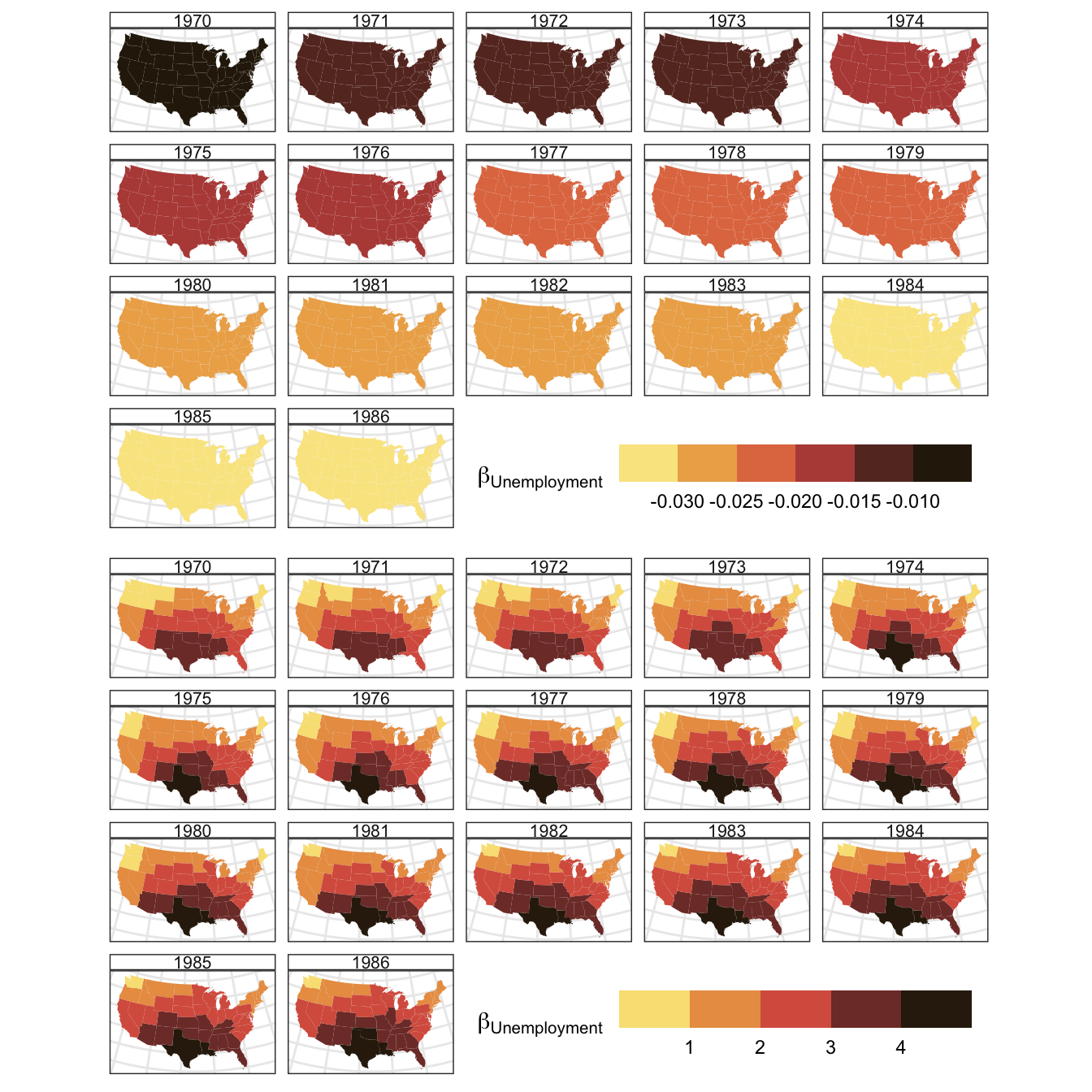
Figure 3.2: The spatial variation of coefficient estimatess for BMA Unemployment and Public captial over time, generated Bayesian Model Avaergaing approach.
3.7 Further info
An R package has been created to do all of this called stgam. It can be downloaded and installed as follows:
It has two vignettes both based around the contents of this workshop: an introduction
And a vignette for undertaking model selection and Bayesian Model Averaging:
Further references to this approach are found to be found in Comber et al. (submitted) with the foundational work described in Comber, Harris, and Brunsdon (2023), Brunsdon, Harris, and Comber (2023) and Comber, Harris, and Brunsdon (2024), and at some point soon the paper describing the stgam package with formal description of the approach (ie with equations) will be submitted to the Journal of Statistical Software (https://www.jstatsoft.org/).