Chapter 2 SVCs and TVCs with GGP-GAMs
In this session you will:
- Create and interpret a simple SVC using GAMs with GP smooths.
- Create and interpret a simple TVC GAM.
- Extend this to a GP GAM that includes both space and time in smooths to define a STVC model.
- Be encourages to reflect on how space and time interact and the assumptions embedded in the model specification.
You should make sure the data and required packages are loaded as in Session 1
# load the packages
library(tidyverse)  # for data manipulation and plotting
library(sf)         # for spatial data
library(mgcv)       # for GAMs
library(cols4all)   # for nice shading in graphs and maps
library(cowplot)    # for managing plots
# load the data
load("us_st_data.RData")
The key ideas underpinning the development of SVCs with GAMs in this section are:
- Standard linear regression assumes that predictor-to-response relationships to be the same throughout the study area.
- This is often not the case when when location is considered for example of outliers
- Many geographic processes have a Gaussian form when they are examined over 2-dimensional space, as they essentially exhibit distance decay.
- The splines introduced in Part 1 can be of different forms. One such form is a Gaussian Process (GP) spline.
- GP splines can be specified to model non-linearity (wiggliness) over geographic space if location is included with the covariate.
- A GAM with GP splines parameterised by location - a Geographic GP GAM or GGP-GAM - defines a spatially varying coefficient (SVC) model
The approach is presented in outline below, but detail of the SVCs, TVCs and STVCs constructed using GAMs with GP smooths, and the evolution of their application from spatial models to space-time coefficient modelling can be found in Comber, Harris, and Brunsdon (2024) and Comber et al. (submitted). In this, the concept of a Gaussian Process (Wood 2020) is important in the context of regression modelling. It provides a data model of the likelihood that a given data set is generated given a statistical model involving some unknown parameters and in regression modelling, the unknown parameters are the regression parameters. These are described formally in Comber, Harris, and Brunsdon (2024) and Comber et al. (submitted).
2.1 A simple SVC
A spatially varying coefficient model will be created using the productivity data contained in the produc object that was loaded earlier. As well as productivity related attributes, this data set contains locational information of the state geometric centroid locations under a USA Contiguous Equidistant Conic projection (ESRI:102005) (see Table 1.1 in the first session). The code below maps X and Y locations along with the US state areas in us_data as in Figure 2.1.
ggplot() +  geom_sf(data = us_data, fill = NA) +
  geom_point(data = produc |> filter(year == "1970"), aes(x = X, y = Y)) +
  theme_bw() + ylab("") + xlab("")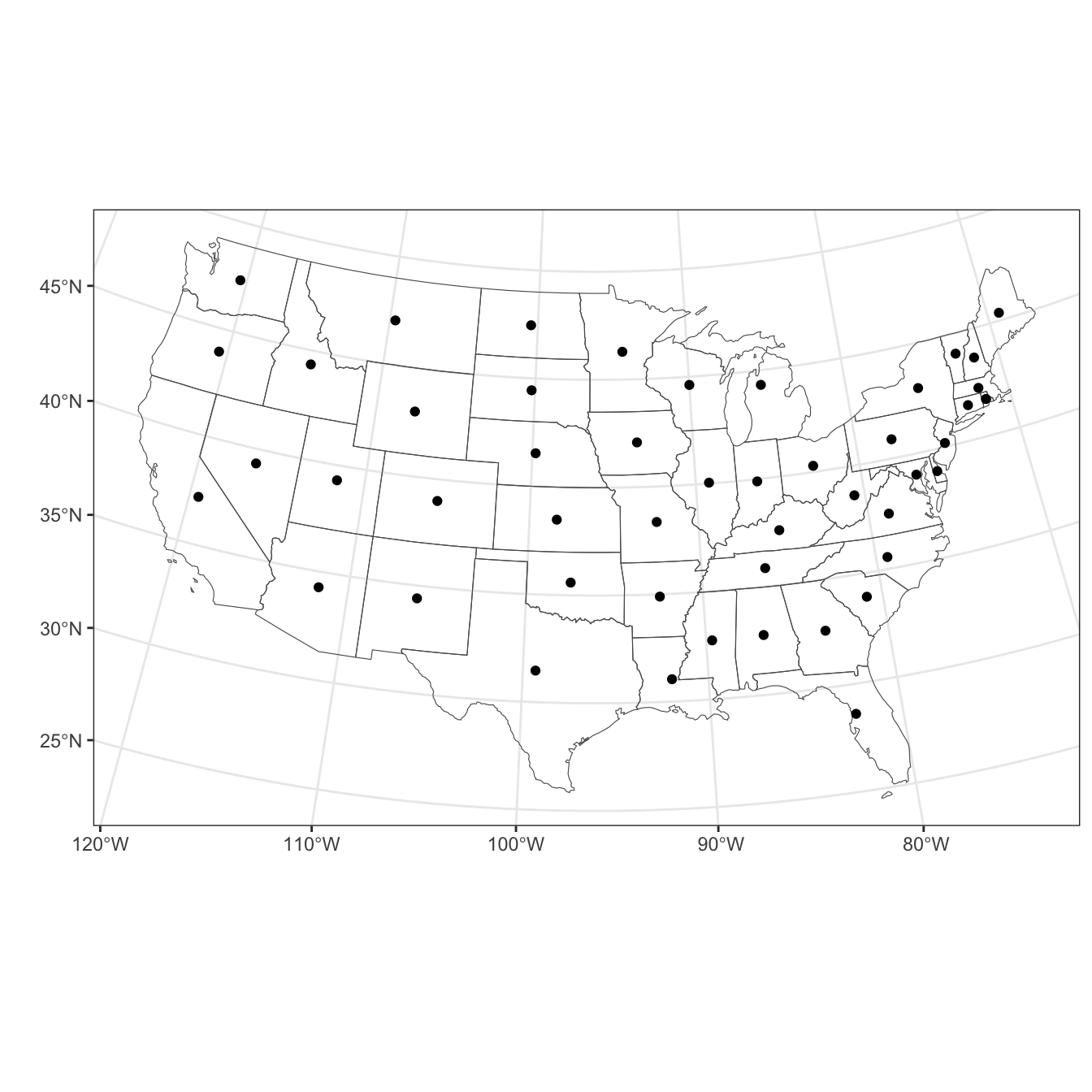
Figure 2.1: The US States and the geoemtric centroids used as locations in the SVC and STVC models.
The initial aim is to calibrate an SVC model of the relationship between Private capital stock (privC), the target variable, with Unemployment (unemp) and Public capital (pubC) covariates, where the spatial coefficient functions are assumed to be realisation of a Gaussian Process (GP) introduced above. Essentially this extends the standard regression models from the first session into the spatial case.
The code below defines an intercept column (int) in the data. This to allow the intercept to be treated as an addressable term in the model. It also defines parametric and non-parametric forms for the intercept and each covariate, so that they can can take a a global form (i.e. as in a standard OLS regression) and a spatially varying form in the GP smooth.
# define intercept term
produc <- produc |> mutate(int = 1)
# create the SVC
svc.gam = gam(privC ~ 0 +
                int   + s(X, Y, bs = 'gp', by = int) +
                unemp + s(X, Y, bs = "gp", by = unemp) +
                pubC  + s(X, Y, bs = "gp", by = pubC),
              data = produc |> filter(year == "1970"))
Notice the 0 + in the model. This indicates that the intercept coefficient is not included implicitly and it is included explicitly as int. Also notice the different form of the splines from those specified in Part 1. Here, for each covariate, a GP smooth is specified for X and Y (the coordinates in geographic space) and the covariate is included via the by parameter. This is to explore the interaction of the covariate with the target variable over the space defined by X and Y locations, allowing spatially varying coefficients to be generated. The model has 4 key terms specified in the same way by <VAR> + (X, Y, b s= 'gp', by = <VAR>):
- the
<VAR>is the fixed parametric term for the covariate s(...)defines the smoothbs = 'gp'states that this is a GP smoothby = <VAR>suggests the GP should be multiplied by variable
The model output can be assessed: the k' and edf parameters are quite close, but the p-values are high and and the k-index is greater than 1 so this looks OK. The diagnostic plots are again generated by the gam.check function as in Figure 2.2:
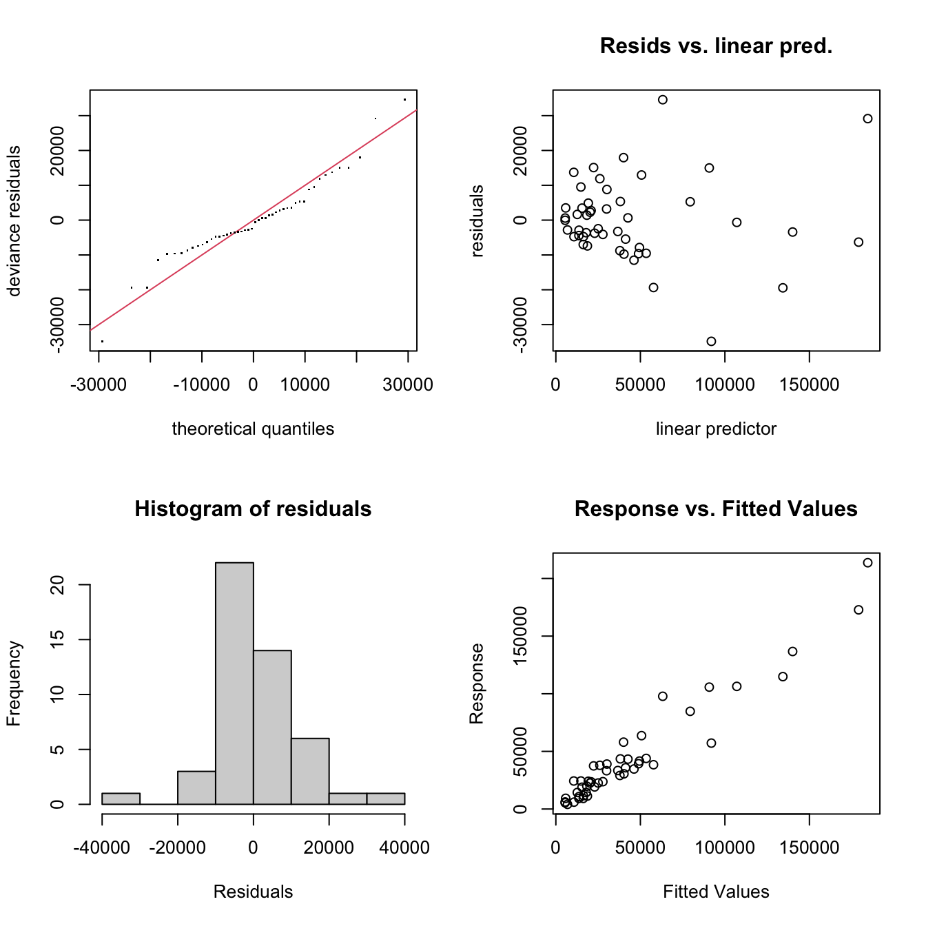
Figure 2.2: The GAM GP SVC diagnostic plots.
##
## Method: GCV   Optimizer: magic
## Smoothing parameter selection converged after 6 iterations by steepest
## descent step failure.
## The RMS GCV score gradient at convergence was 2452.878 .
## The Hessian was not positive definite.
## Model rank =  8 / 101
##
## Basis dimension (k) checking results. Low p-value (k-index<1) may
## indicate that k is too low, especially if edf is close to k'.
##
##                 k'   edf k-index p-value
## s(X,Y):int   32.00  2.00    0.82   0.050 *
## s(X,Y):unemp 33.00  2.00    0.82   0.030 *
## s(X,Y):pubC  33.00  3.67    0.82   0.045 *
## ---
## Signif. codes: 0 '***' 0.001 '**' 0.01 '*' 0.05 '.' 0.1 ' ' 1##
## Family: gaussian
## Link function: identity
##
## Formula:
## privC ~ 0 + int + s(X, Y, bs = "gp", by = int) + unemp + s(X,
## Y, bs = "gp", by = unemp) + pubC + s(X, Y, bs = "gp", by = pubC)
##
## Parametric coefficients:
## Estimate Std. Error t value Pr(>|t|)
## int 0.0014245 0.0003432 4.151 0.000168 ***
## unemp 0.0064540 0.0015548 4.151 0.000168 ***
## pubC -3.9243042 0.9571325 -4.100 0.000196 ***
## ---
## Signif. codes: 0 '***' 0.001 '**' 0.01 '*' 0.05 '.' 0.1 ' ' 1
##
## Approximate significance of smooth terms:
## edf Ref.df F p-value
## s(X,Y):int 2.000 2.000 0.453 0.639
## s(X,Y):unemp 2.000 2.000 0.405 0.676
## s(X,Y):pubC 3.672 3.715 188.593 <2e-16 ***
## ---
## Signif. codes: 0 '***' 0.001 '**' 0.01 '*' 0.05 '.' 0.1 ' ' 1
##
## Rank: 8/101
## R-sq.(adj) = 0.918 Deviance explained = 96.5%
## GCV = 1.9338e+08 Scale est. = 1.613e+08 n = 48Here it can be seen that
- the model is well tuned: all of the all effective degrees of freedom (
edfare well belowkin thegam.check()printed output (thek-index<1issue is not important because of this) - all of the the fixed parametric terms are significant
- of the smooth terms, only
pccapis locally significant and spatially varying.
The spatially varying coefficient estimates can be extracted using predict. To do this a dummy data set is created with the pubC term set to 1, and the intersect and unemp terms set to zero. The result is that the predicted values for the coefficient estimate are just a function of \(\beta_2\), the pubC coefficient estimate at each location.
get_b2<- produc |> filter(year == "1970") |> mutate(int = 0, unemp = 0, pubC = 1)
res <- produc |> filter(year == "1970") |>
  mutate(b2 = predict(svc.gam, newdata = get_b2))
The resulting data.frame called res has a new variable called b2 which is the spatially varying coefficient estimate for pubC. For comparison, we can generate the spatially varying coefficient estimate for the intercept (\(\beta_0\)) and unemp \(\beta_1\) (which were not found to be significant locally) in the same way by setting the other terms in the model to zero:
get_b0 <- produc |> filter(year == "1970") |> mutate(int = 1, unemp = 0, pubC = 0)
res <- res |> mutate(b0 = predict(svc.gam, newdata = get_b0))
get_b1 <- produc |> filter(year == "1970") |> mutate(int = 0, unemp = 1, pubC = 0)
res <- res |> mutate(b1 = predict(svc.gam, newdata = get_b1))
So res has the records for the year 1970 and three new columns for b0, b1 and b2 The distribution of the spatially varying coefficient estimates can be examined:
##                b0       b1    b2
## Min.    -19058.71 -2848.15 -0.18
## 1st Qu.  -7882.46 -1199.14  1.29
## Median     731.22  -156.64  2.11
## Mean         0.00     0.30  2.08
## 3rd Qu.   7891.22  1179.57  2.85
## Max.     20699.80  3362.89  3.80
And standard dplyr and ggplot approaches can be used to join and map them, formally \(\beta_0\), \(\beta_1\) and \(\beta_2\)) as in Figure 2.3. Notice the North-South trend for the Intercept and the East-West and trend for Unemployment - both insignificant predictors of privC - and a much stronger specific spatial pattern between the target variable and Public capital (pubC), with particularity high coefficient estimates in the south.
# join the data
map_results <-
  us_data |> left_join(res |> select(GEOID, b0, b1, b2), by = "GEOID")
# plot the insignificant coefficient estimates
tit =expression(paste(""*beta[0]*""))
p1 <-
  ggplot(data = map_results, aes(fill=b0)) +
  geom_sf() +
  scale_fill_continuous_c4a_div(palette="brewer.spectral",name=tit) +
  coord_sf() +
  ggtitle("Intercept: not significant")
tit =expression(paste(""*beta[1]*""))
p2 <-
  ggplot(data = map_results, aes(fill=b1)) +
  geom_sf() +
  scale_fill_continuous_c4a_div(palette="brewer.spectral",name=tit) +
  coord_sf() +
  ggtitle("Unemployment: not significant")
# plot the significant pubC coefficient estimates
tit =expression(paste(""*beta[2]*" "))
p3 <-
  ggplot(data = map_results, aes(fill=b2)) +
  geom_sf() +
  scale_fill_continuous_c4a_div(palette="brewer.prgn",name=tit) +
  coord_sf() +
  ggtitle("Public captial: significant")
plot_grid(p1, p2, p3, ncol = 1)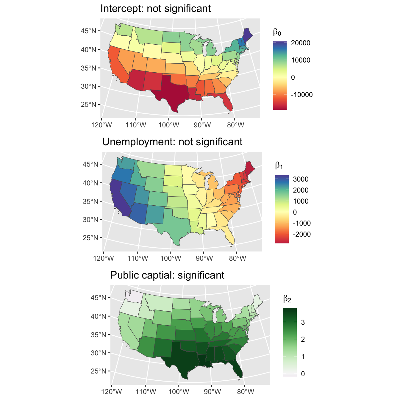
Figure 2.3: The Intercept, Unemployment and Public capital spatially varying coefficient estimates.
2.2 A simple TVC
Thus far all of the analyses have used the data filter for 1970 for the 48 states, whose X-Y location was used to parametrise a Gaussian Process smooth to create the SVCs. The same structure can be used to create a temporally vary coefficient model (TVC), with smooths specified to include the year parameter, but this time not restricting the analysis data to records from a single year:
# create the TVC
tvc.gam = gam(privC ~ 0 +
                int   + s(year, bs = 'gp', by = int) +
                unemp + s(year, bs = "gp", by = unemp) +
                pubC  + s(year, bs = "gp", by = pubC),
              data = produc)
The model can be inspected in the same way to examine the the k' and edf parameters using the gam.check function and again there are no concerns:
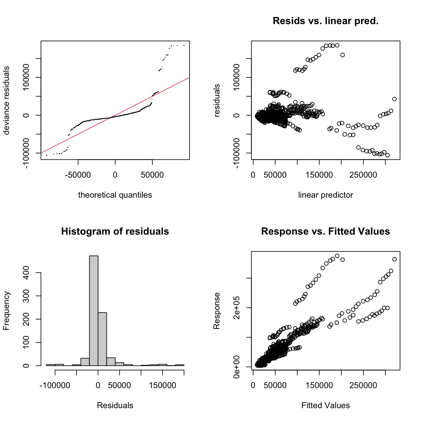
Figure 2.4: The GAM GP TVC diagnostic plots.
##
## Method: GCV   Optimizer: magic
## Smoothing parameter selection converged after 12 iterations.
## The RMS GCV score gradient at convergence was 27.53856 .
## The Hessian was positive definite.
## Model rank =  36 / 38
##
## Basis dimension (k) checking results. Low p-value (k-index<1) may
## indicate that k is too low, especially if edf is close to k'.
##
##                 k'  edf k-index p-value
## s(year):int   11.0  1.0    1.07    0.95
## s(year):unemp 12.0  1.5    1.07    0.98
## s(year):pubC 12.0 1.5 1.07 0.97##
## Family: gaussian
## Link function: identity
##
## Formula:
## privC ~ 0 + int + s(year, bs = "gp", by = int) + unemp + s(year,
## bs = "gp", by = unemp) + pubC + s(year, bs = "gp", by = pubC)
##
## Parametric coefficients:
## Estimate Std. Error t value Pr(>|t|)
## int 1.636e+04 3.439e+03 4.756 2.34e-06 ***
## unemp -4.753e+02 2.606e+02 -1.824 0.0685 .
## pubC 9.220e-01 1.849e-02 49.880 < 2e-16 ***
## ---
## Signif. codes: 0 '***' 0.001 '**' 0.01 '*' 0.05 '.' 0.1 ' ' 1
##
## Approximate significance of smooth terms:
## edf Ref.df F p-value
## s(year):int 1.0 1.0 10.30 0.00138 **
## s(year):unemp 1.5 1.5 5.77 0.00460 **
## s(year):pubC 1.5 1.5 1092.60 < 2e-16 ***
## ---
## Signif. codes: 0 '***' 0.001 '**' 0.01 '*' 0.05 '.' 0.1 ' ' 1
##
## Rank: 36/38
## R-sq.(adj) = 0.771 Deviance explained = 88.3%
## GCV = 8.2539e+08 Scale est. = 8.1932e+08 n = 816The model summary indicates that all of the parametric and temporally vary coefficients are significant at the 95% level except the parametric one for Unemployment, but there are some interesting patterns in the residuals, as reflected in the diagnostics plots in Figure 2.4 and the model fit (\(R^2\)) value.
The temporally varying coefficients can be extracted in the same way as the DVC approach, explored using the predict function and setting each of the covariates to 1 and the others to zero in turn:
get_b0<- produc |> mutate(int = 1, unemp = 0, pubC = 0)
res <- produc |> mutate(b0 = predict(tvc.gam, newdata = get_b0))
get_b1 <- produc |> mutate(int = 0, unemp = 1, pubC = 0)
res <- res |> mutate(b1 = predict(tvc.gam, newdata = get_b1))
get_b2 <- produc |> mutate(int = 0, unemp = 0, pubC = 1)
res <- res |> mutate(b2 = predict(tvc.gam, newdata = get_b2))
The variation in coefficient estimates can be inspected over time, remembering that each State has the same coefficient estimate value for each year. Notice the linear changes due to the linearity of the time covariate in Figure 2.5.
res |>
  filter(state == "ARIZONA") |>
  select(year, b0, b1, b2) %>%
  pivot_longer(-year) %>%
  ggplot(aes(x = year, y = value)) +
  geom_point() + geom_line() +
  facet_wrap(~name, scale = "free") +
theme_bw() + xlab("Year") + ylab("") 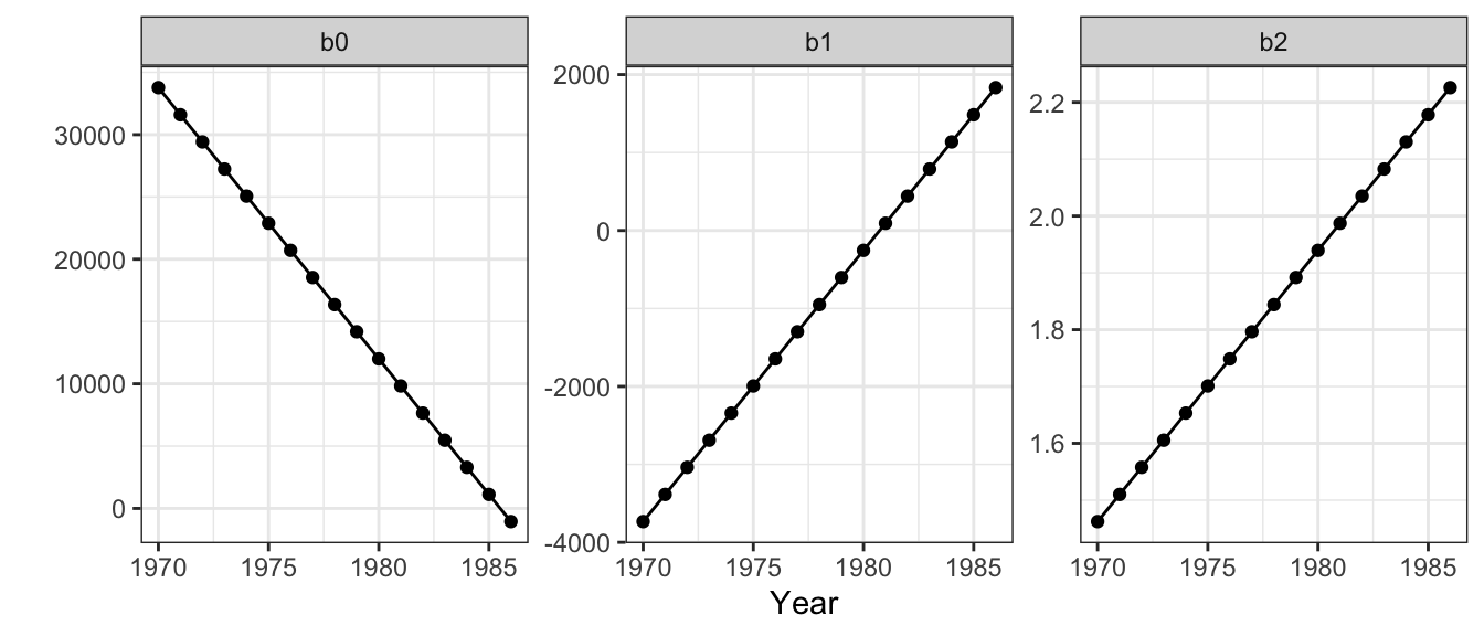
Figure 2.5: Trends in the temporally varying coefficient estimates.
2.3 Spatially and Temporally Varying Coefficient (STVC) models
We can combine space and time in GAM GP splines. But how? We could use separate smooths for location and for time, or a single, 3D smooth parameterised with both location and time. There are assumptions associated with each of these. Separate smooths assumes that spatial and temporal trends do not interact, that any temporal variations in the predictor-target variable relationships are independent of location. A single combined spline assumes that spatial and temporal processes do interact and that the temporal trends in predictor-target variable relationships will vary with location.
The code below specifies the interaction of the covariates within a single space-time GP smooth. You will notice this takes a few seconds longer to run, and choice of how to specify the smooths is explored in the Additional Work section below.
stvc.gam = gam(privC ~ 0 +
                 int   + s(X, Y, year, bs = 'gp', by = int) +
                 unemp + s(X, Y, year, bs = "gp", by = unemp) +
                 pubC  + s(X, Y, year, bs = "gp", by = pubC),
               data = produc)
The model can be inspected in the usual way using the gam.check function (again, no concerns) and the summary function with \(k\) and \(edf\) despite the concerning k-index and p-value values. In this case all of the parametric and smooth coefficient estimates are significant at the 95% level, and the model fit (\(R^2\)) has again increased over the SVC model.
The coefficients spatial and temporally vary coefficients can be extracted in the same way as before
get_b0<- produc |> mutate(int = 1, unemp = 0, pubC = 0)
res <- produc |> mutate(b0 = predict(stvc.gam, newdata = get_b0))
get_b1 <- produc |> mutate(int = 0, unemp = 1, pubC = 0)
res <- res |> mutate(b1 = predict(stvc.gam, newdata = get_b1))
get_b2 <- produc |> mutate(int = 0, unemp = 0, pubC = 1)
res <- res |> mutate(b2 = predict(stvc.gam, newdata = get_b2))
The variation in coefficient estimates from this STVC-GAM model over the 48 US states over 17 years can be summarised using the code below which indicates that a positive relationship between Private capital (b2) with with Public capital and a mixed positive and negative one with Unemployment (b1) and the Intercept (b0).
It is instructive to unpick some of the model coefficients in more detail and the code below summarises variations over time through the median values of each coefficient estimate:
res |> select(year, b0, b1, b2) |>
  group_by(year) |>
  summarise(med_b0 = median(b0),
            med_b1 = median(b1),
            med_b2 = median(b2))
## # A tibble: 17 × 4
## year med_b0 med_b1 med_b2
## <int> <dbl> <dbl> <dbl>
## 1 1970 -77.8 -313. 1.95
## 2 1971 -77.8 -313. 1.99
## 3 1972 -77.8 -313. 2.03
## 4 1973 -77.8 -313. 2.07
## 5 1974 -77.8 -313. 2.11
## 6 1975 -77.8 -313. 2.15
## 7 1976 -77.8 -313. 2.19
## 8 1977 -77.8 -313. 2.23
## 9 1978 -77.8 -313. 2.27
## 10 1979 -77.8 -313. 2.31
## 11 1980 -77.8 -313. 2.35
## 12 1981 -77.8 -313. 2.39
## 13 1982 -77.8 -313. 2.43
## 14 1983 -77.8 -313. 2.47
## 15 1984 -77.8 -313. 2.51
## 16 1985 -77.8 -313. 2.55
## 17 1986 -77.8 -313. 2.59It is evident that of the 2 covariates and the intercept used to model Private capital, only Public capital (b2) varies (increases) over time. This increase is shown visually in Figure 2.6.
# inputs to plot
res |> select(starts_with("b"), year) |>
  mutate(year = "All Years") -> tmp
cols = c(c4a("tableau.red_gold", n = 17, reverse = T), "grey")
tit =expression(paste(""*beta[`Private Capital`]*""))
# plot
res |> select(starts_with("b"), year) |>
  rbind(tmp) |>
  mutate(year = factor(year)) |>
  ggplot(aes(y = year, x = b2, fill = year)) +
  geom_boxplot(outlier.alpha = 0.1) +
  scale_fill_manual(values=cols, guide = "none") +
theme_bw() + xlab(tit) + ylab("Time") 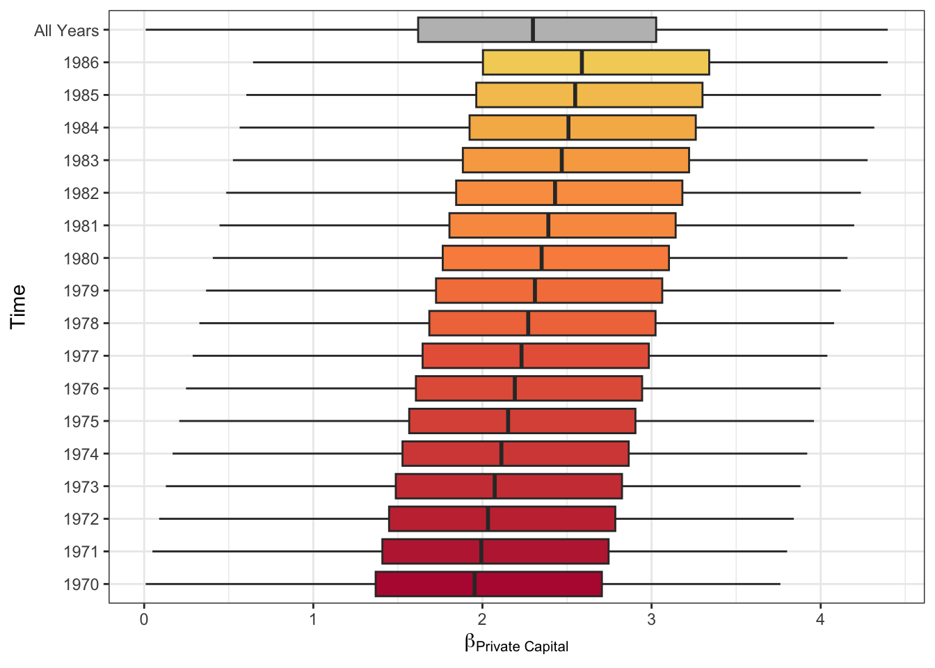
Figure 2.6: The temporal variation of the Public capital coefficient estimates over 17 years.
The spatial pattern of this temporal trend can also be explored as in Figure 2.7. This shows that the increasing intensity of the effect of Public capital on Private capital does not vary spatially: the increase in effect is spatially even, with high values in the south.
tit =expression(paste(""*beta[`Public Capital`]*""))
# join the data
map_results <-
  us_data |> left_join(res |> select(GEOID, year, b0, b1, b2), by = "GEOID")
# create the plot
map_results |>
  ggplot() + geom_sf(aes(fill = b2), col = NA) +
    scale_fill_binned_c4a_seq(palette="scico.lajolla", name = tit) +
  facet_wrap(~year) +
    theme_bw() + xlab("") + ylab("") +
    theme(
      strip.background =element_rect(fill="white"),
      strip.text = element_text(size = 8, margin = margin()),
      legend.position = c(.7, .1),
      legend.direction = "horizontal",
      legend.key.width = unit(1, "cm"),
        axis.title.x=element_blank(),
        axis.text.x=element_blank(),
        axis.ticks.x=element_blank(),
        axis.title.y=element_blank(),
        axis.text.y=element_blank(),
axis.ticks.y=element_blank()) 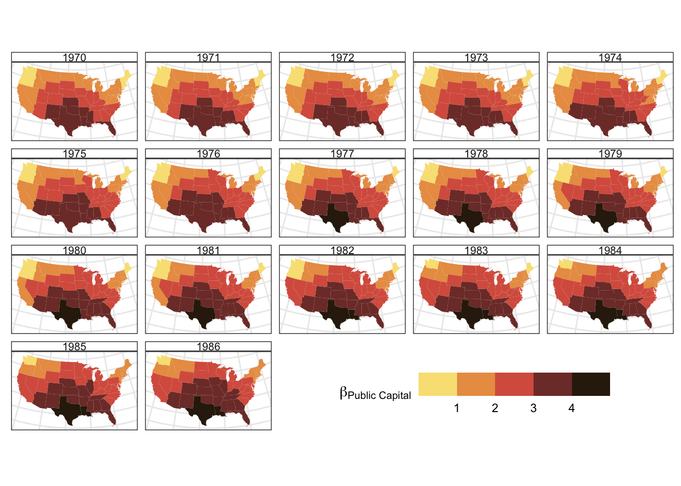
Figure 2.7: The spatial variation of the Unemployment coefficient estimates over time.
2.4 Further Work
The STCV model specified above include space and time in a single splines for each the covariates. This is to assume that that spatial and temporal processes do interact and that the temporal trends in predictor-target variable relationships will vary with location. But is this assumption correct? The next section – if you have time – creates different models, with different assumptions, and evaluates them to determine which one or set fo models is / are the most probable.
2.5 Summary
The rationale for using GAMs with GP splines for spatially varying coefficient (SVC) or temporally varying coefficient (TVC) models is as follows:
- GAMs with splines or smooths capture non-linear relationships between the response variable and covariates.
- splines generate a varying coefficient model when they are parameterised with more than one variable.
- this is readily extending to the temporal and / or spatial dimensions to generate SVCs, TVCs and STVCs.
- different splines are available, but GP splines reflect Tobler’s First Law of geography (spatial autocorrelation, process spatial heterogeneity, etc).
- this can be extended to the temporal case on the assumption of temporal decay (similarity decreases over time).
- GAMs are robust, have a rich theoretical background and been subject to much development.
Initial research has demonstrated the formulation and application of a GAM with GP splines calibrated via observation location as a multiscale SVC model: the Geographical Gaussian Process GAM (GGP-GAM) (Comber, Harris, and Brunsdon 2024). The GGP-GAM was compared with the most popular SVC model, Geographically Weighted Regression (GWR) (Brunsdon, Fotheringham, and Charlton 1996) and shown to out-perform Multiscale GWR.
However, when handling space and time, simply plugging all the space time data into specific GAM configuration is to make potentially unreasonable assumptions about how space and time interact in spatially and temporally varying coefficient (STVC) models. To address this workshop has suggested that the full set of models is investigated to identify the best model or the best set of models. Where there is a clear winner, this can be applied. Where these is not, as in the example used then the model coefficients can be combined using Bayesian Model Averaging.