Chapter 1 GAM with Splines
In this session you will:
- Set up your RStudio session, loading data and packages
- Undertake and unpick a standard GAM regression
- Extend this to a GAM with splines (also referred to as “smooths”)
1.1 Data and Packages
The first code chuck loads the packages required, checking for the presence on your computer and installing them if necessary. Remember that you can execute chunks of code by highlighting it and clicking the Run button, or by placing your cursor inside it and pressing Cmd+Shift+Enter.
# package list
packages <- c("tidyverse","sf", "mgcv", "cols4all", "cowplot")
# check which packages are not installed
not_installed <- packages[!packages %in% installed.packages()[, "Package"]]
# install missing packages
if (length(not_installed) > 1) {
  install.packages(not_installed, repos = "https://cran.rstudio.com/", dep = T)
}
# load the packages
library(tidyverse)  # for data manipulation and plotting
library(sf)         # for spatial data
library(mgcv)       # for GAMs
library(cols4all)   # for nice shading in graphs and maps
library(cowplot)    # for managing plots
Next load some some data. This is annual economic productivity data for the 48 contiguous US states (with Washington DC merged into Maryland), for years 1970 to 1985 (17 years). The data productivity data table was extracted from the plm package (Croissant, Millo, and Tappe 2022) and it is described in Table 1.1. The code below also loads a spatial dataset of the US states from the spData package (Bivand, Nowosad, and Lovelace 2019).
# from https://www.dropbox.com/scl/fi/rt69d7v1f7beov0oz643o/us_st_data.RData?rlkey=am69voqglrfnjw3pkhlvhg0yj&dl=1
# from Lex's dropbox
download.file("https://shorturl.at/UYQ2Q", destfile = "us_st_data.RData")
load("us_st_data.RData")
head(produc)
## state GEOID year region pubC hwy water util privC gsp emp unemp
## 1 ALABAMA 01 1970 6 15032.67 7325.80 1655.68 6051.20 35793.80 28418 1010.5 4.7
## 2 ALABAMA 01 1971 6 15501.94 7525.94 1721.02 6254.98 37299.91 29375 1021.9 5.2
## 3 ALABAMA 01 1972 6 15972.41 7765.42 1764.75 6442.23 38670.30 31303 1072.3 4.7
## 4 ALABAMA 01 1973 6 16406.26 7907.66 1742.41 6756.19 40084.01 33430 1135.5 3.9
## 5 ALABAMA 01 1974 6 16762.67 8025.52 1734.85 7002.29 42057.31 33749 1169.8 5.5
## 6 ALABAMA 01 1975 6 17316.26 8158.23 1752.27 7405.76 43971.71 33604 1155.4 7.7
## X Y
## 1 858146.3 -647095.8
## 2 858146.3 -647095.8
## 3 858146.3 -647095.8
## 4 858146.3 -647095.8
## 5 858146.3 -647095.8
## 6 858146.3 -647095.8## Simple feature collection with 48 features and 6 fields
## Geometry type: GEOMETRY
## Dimension: XY
## Bounding box: xmin: -2361579 ymin: -1486010 xmax: 2256096 ymax: 1399644
## Projected CRS: USA_Contiguous_Equidistant_Conic
## # A tibble: 48 × 7
## GEOID NAME REGION AREA total_pop_10 total_pop_15 geometry
## * <chr> <chr> <fct> [km^2] <dbl> <dbl> <GEOMETRY [m]>
## 1 01 ALABAMA South 133709. 4712651 4830620 POLYGON ((719392.5 -424686…
## 2 04 ARIZONA West 295281. 6246816 6641928 POLYGON ((-1754060 -526705…
## 3 08 COLORADO West 269573. 4887061 5278906 POLYGON ((-1106674 176454.…
## 4 09 CONNECTICUT Norteast 12977. 3545837 3593222 POLYGON ((1852498 484017.5…
## 5 12 FLORIDA South 151052. 18511620 19645772 MULTIPOLYGON (((1478511 -1…
## # ℹ 43 more rows| Variable | Description |
|---|---|
| gsp | Gross State Products the private business output (productivity) |
| emp | Labour input measured by the employment in non-agricultural payrolls |
| unemp | State unemployment rate capture elements of the business cycle |
| privC | Private capital stock computed by apportioning Bureau of Economic Analysis (BEA) national stock estimates |
| pubC | Public capital which is composed of highways and streets (hwy) water and sewer facilities (water) and other public buildings and structures (util) |
| X | Easting in metres from USA Contiguous Equidistant Conic projection (ESRI:102005) |
| Y | Northing in metres from USA Contiguous Equidistant Conic projection (ESRI:102005) |
1.2 Regression
The standard form for a linear regression, which are commonly solved using an ordinary least squares approach (OLS) is:
\[y = \beta_{0} + \sum_{m}^{k=1}\beta_{k}x_{k} + \epsilon \]
where \(y\) is the response variable, \(x_{k}\) is the value of the \(k^{th}\) predictor variable, \(m\) is the number of predictor variables, \(\beta_0\) is the intercept term, \(\beta_k\) is the regression coefficient for the \(k^{th}\) predictor variable and \(\epsilon\) is the random error term.
We can make an initial model of Private Capital stock (privC) and examines the result:
##
## Call:
## lm(formula = privC ~ unemp + pubC, data = filter(produc, year ==
##     1970))
##
## Residuals:
##    Min     1Q Median     3Q    Max
## -41801  -8859  -4389   1641 118082
##
## Coefficients:
##               Estimate Std. Error t value Pr(>|t|)
## (Intercept) 17388.6616 14901.5959   1.167    0.249
## unemp       -1224.9397  3006.9595  -0.407    0.686
## pubC            1.5585     0.1389  11.217 1.26e-14 ***
## ---
## Signif. codes:  0 '***' 0.001 '**' 0.01 '*' 0.05 '.' 0.1 ' ' 1
##
## Residual standard error: 23090 on 45 degrees of freedom
## Multiple R-squared:   0.74,  Adjusted R-squared:  0.7284
## F-statistic: 64.04 on 2 and 45 DF,  p-value: 6.873e-14
We have a model with a good \(R^2\) value, describing the relationship between the different covariates and Private capital. And the coefficient estimates can be interpreted in the usual way:
- each additional 1% of unemployment, is associated with a $1225 decrease in private capital stock, although not significantly;
- each additional $1 of public capital which (highways, water and sewer facilities, public buildings and structures), is associated with a $1.6 increase private capital stock.
This should all be relatively familiar, and sets the scene for GAMs in the next section.
1.3 GAM Regression
GAMs are Generalised Additive Models. They were originally proposed by Hastie and Tibshirani (1987). The gam function in the mcgv package (S. Wood 2018) can be used to fit a regression model in the same way. The model created by the code below generates the same fixed parametric coefficient estimates as the standard OLS model above, and leading to the same interpretations:
##
## Family: gaussian
## Link function: identity
##
## Formula:
## privC ~ unemp + pubC
##
## Parametric coefficients:
##               Estimate Std. Error t value Pr(>|t|)
## (Intercept) 17388.6616 14901.5959   1.167    0.249
## unemp       -1224.9397  3006.9595  -0.407    0.686
## pubC            1.5585     0.1389  11.217 1.26e-14 ***
## ---
## Signif. codes:  0 '***' 0.001 '**' 0.01 '*' 0.05 '.' 0.1 ' ' 1
##
##
## R-sq.(adj) =  0.728   Deviance explained =   74%
## GCV = 5.6877e+08  Scale est. = 5.3322e+08  n = 48
However, GAMs also allow users to examine non-linear relationships through the uses of smooths or splines (more on these later). The basic ideas behind the GAM with smooths framework are that:
- Relationships between the dependent variable and predictor variables follow smooth patterns that can be linear or non-linear
- It is possible to estimate the different components of these smooth relationships individually and simultaneously and then predict or model the target variable by adding them up.
These ideas are illustrated in the figure below from https://multithreaded.stitchfix.com/blog/2015/07/30/gam/:
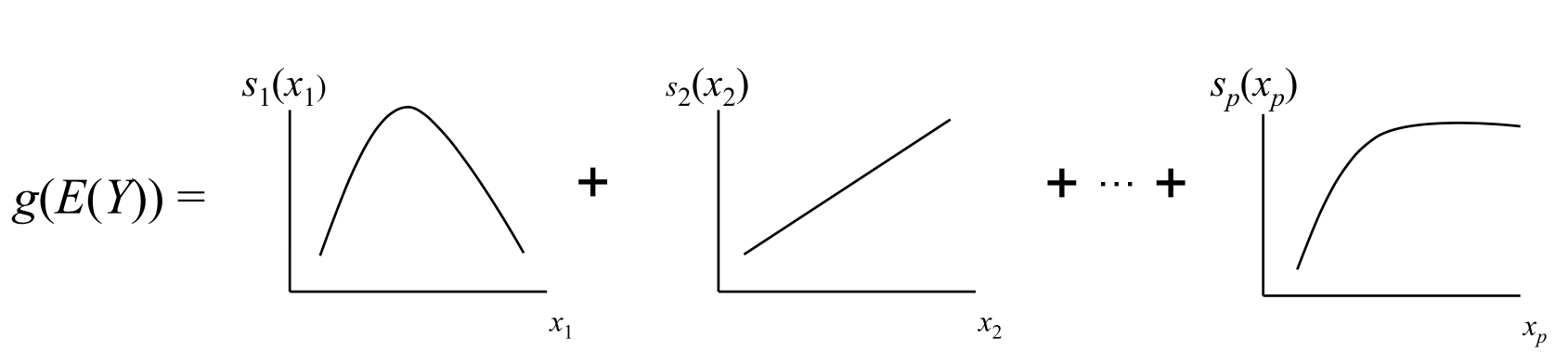
where \(Y\) is the target variable \(E(Y)\) is the expected value, \(g(Y)\) is the link function that links the expected value to the predictor variables \(x_1 \dots x_p\), and the terms \(s_1(x_1), \dots , s_p(x_p)\) indicate the smooth, nonparametric (non-linear) functions.
To illustrate the need for and advantages of GAM based smooths, the code below plots the target variable against the two predictor variables. Here is is evident that the relationships with the target variable are relatively smooth, but importantly that the the assumption of linear relationships estimated under a standard regression may not be appropriate in all cases: if the relationships between the target variable \(y\) and the 2 covariates are examined as in Figure 1.1, then there are perhaps some reasons for concern: although there is a broadly linear and the positive effect for pubC, it is a bit curvy and the relationship with unemp is difficult to characterise in a linear way - it is initially sharply positive for low values, then negative… etc.
produc |>
  filter(year == "1970") |>
  select(privC, unemp, pubC) %>%
  pivot_longer(-privC) %>%
  ggplot(aes(privC, value)) +
  #geom_point(alpha = 0.2) +
  geom_smooth() +
  facet_wrap(~name, scales = "free")
## `geom_smooth()` using method = 'loess' and formula = 'y ~ x'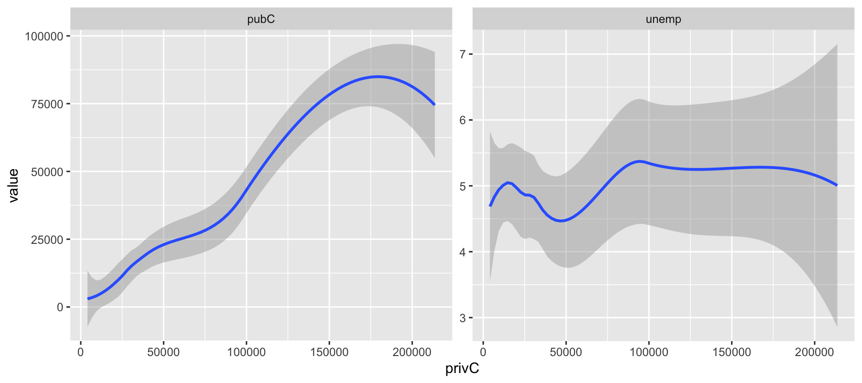
Figure 1.1: Scatterplots of the target variable (private captial stock) with the covariates public capital (pubC) and unemployment (unemp).
This is a very common situation: the assumptions of linearity of a standard linear model are often violated, or the model does not capture the nuances of the data very well. Options for handling this may be to explore non-linear relationships such as polynomial regression with quadratic or cubic terms, or through more complex specifications involving sines or cosines etc. However, these may fail with highly complex relationships, particularly they may fail to capture the true amount of ‘wiggliness’ in the data or they may overfit it. And we frequently have to randomly guess about the form of the relationship until we find a decent model form and associated fits.
To handle these non-linearities GAMs with smooths (also referred to as splines) can be specified.
1.4 Smooths
One way of dealing with any potential non-linearity and wiggliness in the relationship between target and predictor variables, is to is to fit a series of mini models to different parts of the data, in a piecewise way. This can be done by dividing the data into chunks at various points (or knots) along the x-axis, and then fitting a linear or polynomial model to that subset of data. Figure 1.2 shows the a series of linear and quadratic regressions applied to subsets of of the data. These illustrate that there may be different relationships (direction, form) between the target variable and a covariate in different parts of the attribute space.
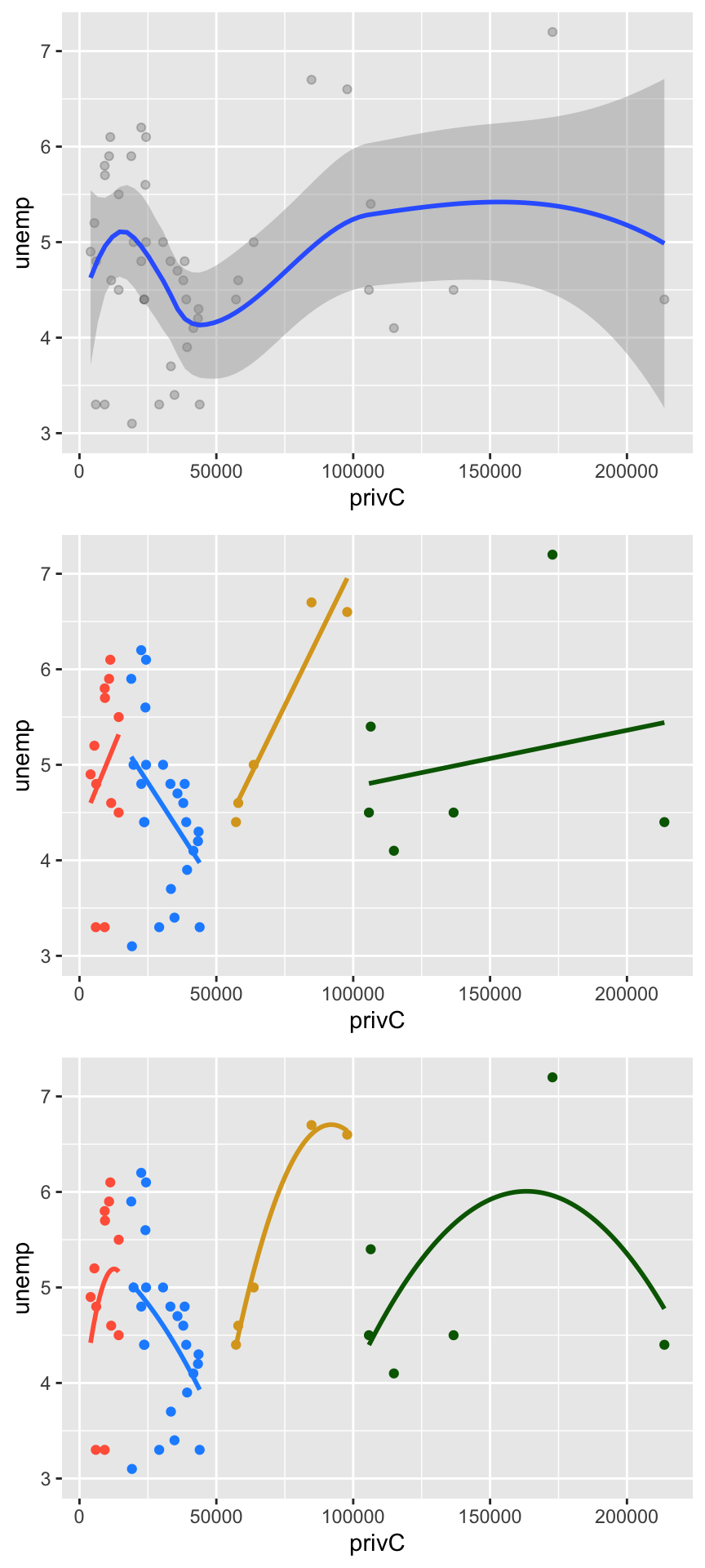
Figure 1.2: Scatterplot of the unemp covariate, original (top), subseted into chunks with ‘within-variable’ linear regression (centre) and quadratic regression (bottom) trend lines.
You can see from the plots above how, for a single variable - recall we are just examining unemp and its relationship with the target variable privC, many different relationships may be present within the data, and how these could be extracted with smooths.
In the plots above, the knots - points at which a within-data local relationships were found - were identified manually and mini-models for each subset were only created in within the code for the plot. However, these ideas of multiple “within the variable” models, underpin the notion of smooths in a Generalized Additive Model. These are illustrated next, and a formal definition is provided in the next session.
1.5 GAMs with Splines
A GAM with smooths can be fitted to the data using the s function:
If the coefficients are examined, it is evident that there is one coefficient for the Intercept as a fixed term, and for each knot in each of the splines. We can see, for example,that the coefficients for both unemp and pubC have a mix of positive and negative slopes in places within the data.
## (Intercept)  s(unemp).1  s(unemp).2  s(unemp).3  s(unemp).4  s(unemp).5  s(unemp).6
##   43897.100  -18148.685   67175.002   -7220.038  -27122.622  -17298.638   15779.132
##  s(unemp).7  s(unemp).8  s(unemp).9   s(pubC).1   s(pubC).2   s(pubC).3   s(pubC).4
##   31434.932  162271.840  -47931.063   14316.940   -5092.109  -57857.938 -110159.419
##   s(pubC).5   s(pubC).6   s(pubC).7   s(pubC).8   s(pubC).9
##  -93588.134   34950.067   44234.494   46093.810   40232.451
These could be examined visually
plot(coef(gam.mod.s)[2:10], col = "red", pch = 16,
    main = "enemp", xlab = "Spline", ylab = "Coefficient")
abline(h = 0, lwd = 2, lty = 2, col = "darkgreen")
# pubC coefficients
plot(coef(gam.mod.s)[11:19], col = "red", pch = 16,
     main = "enemp", xlab = "Spline", ylab = "Coefficient")
abline(h = 0, lwd = 2, lty = 2, col = "darkgreen")
Remember the points in the plots above are slopes. So what we see here is the non-linearity of the relationship between the covariates unemp and pubC with the target variable privC, and in this case, in different parts of the multivariate feature space, the relationships are positive and in others they are negative.
It is possible to check the model to see whether the number of knots has been sufficiently optimised using the gam.check function from the mcgv package. This prints out a summary of these with the effective degrees of freedom (edf) and a number of diagnostic plots: QQ-plot, residuals against predictors, a histogram of residuals and response (\(y\)) vs. fitted values (\(\hat{y})\).
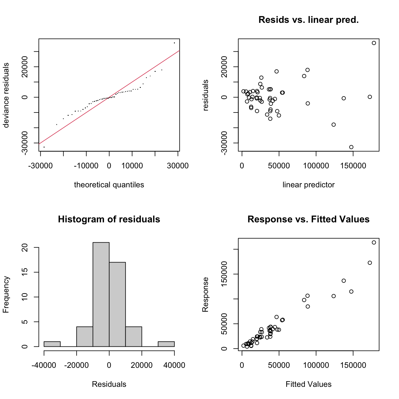
Figure 1.3: Diagnostic plots from the gam.check function.
##
## Method: GCV   Optimizer: magic
## Smoothing parameter selection converged after 13 iterations.
## The RMS GCV score gradient at convergence was 8502.115 .
## The Hessian was positive definite.
## Model rank =  19 / 19
##
## Basis dimension (k) checking results. Low p-value (k-index<1) may
## indicate that k is too low, especially if edf is close to k'.
##
##            k'  edf k-index p-value
## s(unemp) 9.00 6.68    1.13    0.81
## s(pubC)  9.00 8.21    1.31    0.96
Perhaps of most interest is the printed summary of the gam.check function, which indicates the number of knots, \(k\) in each spline / smooth and values for the effective degrees of freedom (edf). The edf values can be interpreted as an indicator of the non-linearity of the relationship of the response (privC) with the predictor variables - i.e. the effective degrees of freedom would have a value of ~1 if the model penalized the smooth term to a near linear relationship. Higher edf values indicate increasing non-linearity in the relationship.
Here all the edf values are less than \(k\) indicating that the model is adequately specified. Here the p-values relate to the knots parameter \(k\) and whether it may be too low, especially if the reported edf is close to the k' value, the maximum possible EDF for the term. These all look OK. S. N. Wood (2017) notes that a “low p-value and a k-index of \(<1\)) may indicate that \(k\) is too low, especially if effective degrees of freedom (EDF) are close to \(k\)”. It is evident that this model is well tuned, but this is not always the case. The key consideration is the distance between the number of knots indicated by k' in the gam.check print out and the effective degrees of freedom. Basically, the edf value should be lower than the \(k\) value for each smooth and this consideration overrides concerns about k-index<1 and low p-values. Here is is evident that the model is well tuned, with 9 knots for each covariate.
In the mcgv package, the parameter which controls the degree of smoothing of the data via spline knots is optimised during GAM fitting. This will be returned to in the context of spatially varying coefficient models with Gaussian Process splines in the next session.
Finally, it is also possible to examine the full summary of the GAM smooth model:
##
## Family: gaussian
## Link function: identity
##
## Formula:
## privC ~ s(unemp) + s(pubC)
##
## Parametric coefficients:
##             Estimate Std. Error t value Pr(>|t|)
## (Intercept)    43897       1778   24.68   <2e-16 ***
## ---
## Signif. codes:  0 '***' 0.001 '**' 0.01 '*' 0.05 '.' 0.1 ' ' 1
##
## Approximate significance of smooth terms:
##            edf Ref.df      F p-value
## s(unemp) 6.677  7.508  2.729  0.0208 *
## s(pubC)  8.214  8.769 39.031  <2e-16 ***
## ---
## Signif. codes:  0 '***' 0.001 '**' 0.01 '*' 0.05 '.' 0.1 ' ' 1
##
## R-sq.(adj) =  0.923   Deviance explained = 94.7%
## GCV = 2.2694e+08  Scale est. = 1.5181e+08  n = 48
This includes a fixed (parametric) coefficient estimate for the Intercept, which can be can be interpreted as linear terms in the model, and summaries of the smooths. The model fit (\(R^2\)) has increased compared to the initial OLS regression models in reg.mod or gam.mod, and the smooth terms (splines) are significant. Here, the p-values relate to the smooths defined over the variable space (in this case s(unemp) and s(pubC)), and their significance can be interpreted as indicating whether they vary within that space. Any insignificant p-values would indicate that although there may be effects, these do not vary locally within this attribute space.
1.6 Summary
The aim of this session was to set the scene by introducing you to GAMs and illustrate their workings. There are some important considerations related to smooths and their knots (\(k\)) but these are generally well optimised by the gam function in the mcgv package.
However the key take home message is that GAM smooths, can be parameterised with a covariate (predictor variable) and is indicative of variation with the space defined by the covariate if this model term is found to be significant.
This starts to suggest how the spline can be further expanded to include location and / or time, and thereby to specify spatially and temporally varying coefficient models. These are detailed in the next session.