Lecture 1 Parameter Estimation

1.1 Overview

In this part we will learn the two most basic inferential methods in statistics, namely Maximum Likelihood Estimation (MLE) in Section 1.3 and the Methods of Moments (MOM) in Section 1.4. We will look at the question, why and how we estimate parameters for given distributions using motivating examples. Last but not least, we will learn what the so-called bias is.

Parameter estimation is essential when fitting a statistical distribution to data. Hence, before we can estimate our parameters, it is to make an assumption about the underlying distribution.

1.2 Example: Coin Flipping

Let’s motivate this topic with a simple coin flip example, where there are two possible outcomes Heads and Tails: \(\Omega = \{H,T\}\). We define the probability of getting Heads as \(p_H\).

1.2.1 Two Coin Flips

You flipped a coin twice, getting Heads once and Tails once. Is this coin fair? What is the estimated probability for Heads on this coin?

Note that you have to revers your thinking from most introductory stats classes: usually, you are asked to give an estimation of the probability of different possible events, given a distribution already equipped with a certain parameter/parameters. Now we want to find out the probability of the events we observed, given different possibilities of parameters. This is how we will find out, which parameter is more likely (for the data at hand).

For the given example, using two different parameter values \(p_H\) the joint probability is calculated as follows:

Fair game (i.e., \(p_H=0.5\)): \[\begin{eqnarray*} P(H,T|p_H=0.5)&\overset{\text{ind.}}{=}&P(H|p_H=0.5) \cdot P(T|p_H=0.5)\\ &=&0.5\cdot 0.5\\ &=&0.25 \end{eqnarray*}\] Unfair game (i.e., \(p_H \neq 0.5\)): \[\begin{eqnarray*} P(H,T|p_H=0.4)&\overset{\text{ind.}}{=}&P(H|p_H=0.4) \cdot P(T|p_H=0.4)\\ &=&0.4\cdot 0.6\\ &=&0.24 \end{eqnarray*}\]

The domain of \(p_H\) reaches from zero (no probability for head) to one (certain that head will come up). Therefore, we can plot the distribution as a function of the parameter while keeping the data fixed:

It can be observed that our data is most likely for a parameter value of \(p_H = 0.5\), which suggests the game is fair.

1.2.2 Three Coin Flips

You flipped a coin three times, getting Heads once and Tails twice. Is this coin fair? What is the estimated probability for Heads on this coin?

We again calculate the joint probabilities for different parameter values:

Fair game (i.e., \(p_H=0.5\)): \[\begin{eqnarray*} P(H, T, T|p_H\!=\!0.5)&\overset{\text{ind.}}{=}&P(H|p_H\!=\!0.5) \cdot P(T|p_H\!=\!0.5) \cdot P(T|p_H\!=\!0.5)\\ &=&0.5\cdot 0.5\cdot 0.5\\ &=&0.125 \end{eqnarray*}\]

Unfair game (i.e., \(p_H \neq 0.5\)): \[\begin{eqnarray*} P(H, T, T|p_H\!=\!0.4)&\overset{\text{ind.}}{=}&P(H|p_H\!=\!0.4) \cdot P(T|p_H\!=\!0.4) \cdot P(T|p_H\!=\!0.4)\\ &=&0.4\cdot 0.6 \cdot 0.6\\ &=&0.144 \end{eqnarray*}\]

The resulting probability distribution for all possible values of \(p_H\) given the data looks as follows:

We find that for the parameter value \(p_H = \frac{1}{3}\) the present data has the highest probability, indicating that the game is not fair.

You can play around with further examples using our coin flip shiny app. Using the app you can exam

1.2.3 Formalization of the Question

In principle, the following questions are identical:

• I flipped my coin \(n\) times and took down the results. What is the probability of flipping Heads with this coin?

• If \(p\) is the probability of Heads: which \(p\) has the highest probability for the coin tosses I observed?

• What does the Maximum-Likelihood-Estimator \(\hat{p}_{\text{ML}}\) look like for the observations \(X_1,\ldots,X_n\)?

In the next section we will translate the question to a mathematical optimization problem.

1.3 Maximum Likelihood Estimation

The Maximum Likelihood Estimation (MLE) is a method used to estimate the parameter of a probability distribution by finding the value that maximizes a so called likelihood function \(L(p)\). This likelihood function represents the joint probability of the observed data as a function of the unknown parameter(s). For a sequence of observations \(X_1, X_2, \ldots, X_n\), it is given by:

\[ \mathcal{L}(p) = \prod_{i=1}^n P(X_i \mid p), \] where \(P(X_i \mid p)\) is the probability of observing \(X_i\) given the parameter \(p\).

1.3.1 Procedure: Bernoulli Distribution

In our coin toss example the independent observations are drawn from a Bernoulli distribution. Thus, the likelihood function becomes:

\[ \mathcal{L}(p) = p^{n_H}(1-p)^{n_T} \]

where \(n_T\) is the number of tails and \(n_H = n-n_T\) is the number of heads in the sample.

To find the MLE for \(\hat{p}_{ML}\) we maximize this likelihood function w.r.t. \(p\): \[\begin{eqnarray*} \hat{p}_{\text{ML}}&=&\underset{p}{\arg\max}\ P(X_1,\ldots,X_n|p)\\ &\overset{\text{ind.}}{=}&\underset{p}{\arg\max}\ \underset{\mathcal{L}(p):= Likelihood}{\underbrace{\prod_{i=1}^n P(X_i|p)}}\\ &\overset{\text{Bernoulli}}{=}&\underset{p}{\arg\max}\ p^{n_H}(1-p)^{n_T}\\ &=&\underset{p}{\arg\max}\ \log\left( p^{n_H}(1-p)^{n_T}\right)\\ &=&\underset{p}{\arg\max}\ \underset{\ell(p):= Log-Likelihood}{\underbrace{ n_H\log p+n_T\log(1-p)}}\\ \end{eqnarray*}\]

Since it is more convenient we derive the log-likelihood according to \(p\): \[\begin{eqnarray*} \frac{d\ell(p)}{dp}&=&\frac{d}{dp}n_H\log p+n_T\log(1-p)\\ &=&\frac{n_H}{p}-\frac{n_T}{1-p} \end{eqnarray*}\] Setting to \(0\): \[\begin{eqnarray*} \frac{n_H}{p}-\frac{n_T}{1-p}&\overset{\text{!}}{=}&0\\ \frac{n_H}{p}&=&\frac{n_T}{1-p}\\ n_Tp&=&n_H(1-p)\\ pn_T+pn_H&=&n_H\\ n_H&=&p\underset{n}{\underbrace{(n_T+n_H)}}\\ \hat{p}_{\text{ML}}&=&\frac{n_H}{n} \end{eqnarray*}\]

1.3.2 Summary: Recipe for MLE

To summarize, we will here present you a detailed recipe for the maximum likelihood estimation:

1. Write down the likelihood function (product of the probability or density function as a function of the parameter of interest)

2. Logarithmize the likelihood function (logarithm of the product becomes the sum of the logarithms) \(\rightarrow\) you now have the log-likelihood

3. Differentiate the log-likelihood according to the parameter of interest

4. Determine the maximum by setting the derivation to zero

There are three main uses cases/arguments for when to use MLE:

• Parameter estimation for modelling
• Comparability due to parametric structures
• Forecasting models

In the next section we will work through this recipe with another example where we find the MLE for both the mean and the variance in the case of the Gaussian distribution.

1.3.3 Example: Mean Google Star Ratings

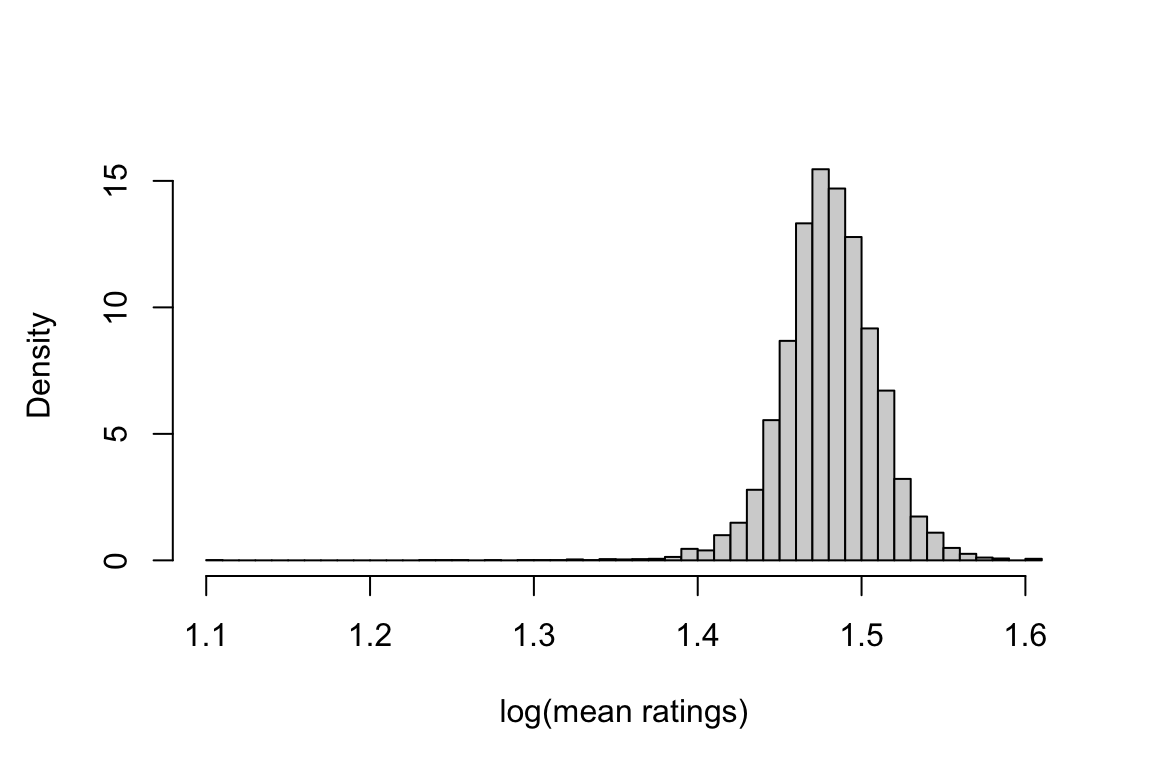
In a second example we will look at a continuous variable, namely the average Google Maps star ratings of different german ZIP codes.

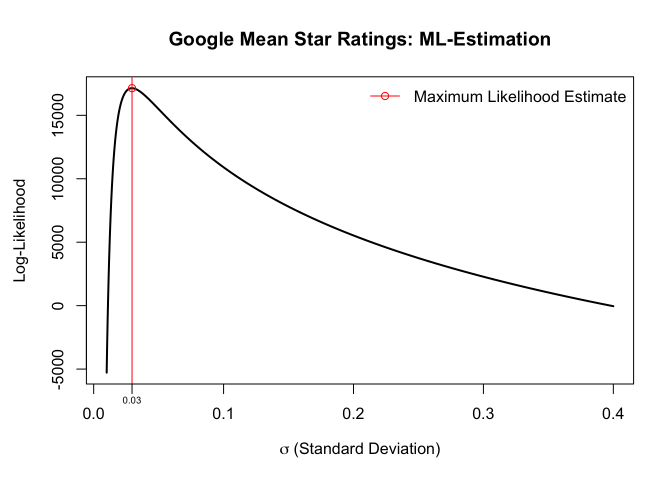
Examining the data suggests that the Gaussian Distribution could be a suitable choice for modeling. We use MLE to find the two parameters involved in this distribution: the mean and the variance.

1.3.3.1 Why Maximum Likelihood Estimation?

In the special case of the Google Star Ratings, there are two additional reasons why we choose MLE:

• Estimation of the mean google rating with calculated impreciseness (MLE for the variance)
• Continuation: predictive variables

1.3.3.2 Derivation: MLE for the Mean

Using the procedure from Section 1.3.2 we obtain the following result for the mean estimate:

\[\hat{\mu}_{\text{ML}} = \frac{1}{n}\sum_{i=1}^n x_i\]

As expected, the result corresponds to the mean value of the data. Now try to derive the result for yourself. The solution can can be found in the dropdown below:

Solution

The probability density function of a normal distribution with mean \(\mu\) and variance \(\sigma^2\) is: \[ f(x_i | \mu, \sigma^2) = \frac{1}{\sqrt{2\pi \sigma^2}} \exp\left(-\frac{(x_i - \mu)^2}{2\sigma^2}\right). \] 1. Write down the likelihood function (product of the probability or density function as a function of the parameter of interest) \[ \mathcal{L}(\mu, \sigma^2) = \prod_{i=1}^n f(x_i | \mu, \sigma^2) = \prod_{i=1}^n \frac{1}{\sqrt{2\pi \sigma^2}} \exp\left(-\frac{(x_i - \mu)^2}{2\sigma^2}\right) \]

2. Logarithmize the likelihood function (logarithm of the product becomes the sum of the logarithms) you now have the log-likelihood:

\[ \begin{align*} \ell(\mu, \sigma^2) &= \log \mathcal{L}(\mu, \sigma^2) \\ &= \sum_{i=1}^n \left[ -\frac{1}{2} \log(2\pi \sigma^2) - \frac{(x_i - \mu)^2}{2\sigma^2} \right] \\ &= -\frac{n}{2} \ln(2\pi \sigma^2) - \frac{1}{2\sigma^2} \sum_{i=1}^n (x_i - \mu)^2 \end{align*} \]

3. Maximize the log-likelihood with respect to the parameter of interest \(\mu\): \[ \begin{align*} \frac{d}{d\mu} \ell(\mu) &= \frac{d}{d\mu} \sum_{i=1}^n (x_i^2 - 2x_i\mu + \mu^2) \\ &= \sum_{i=1}^n (-2x_i + 2\mu) = -2\sum_{i=1}^n x_i + 2n\mu \end{align*} \]

4. Determine the maximum by setting the derivation to zero and solving for \(\mu\): \[ -2\sum_{i=1}^n x_i + 2n\mu \stackrel{!}{=} 0 \\ \implies \hat{\mu}_{\text{ML}} = \frac{1}{n} \sum_{i=1}^n x_i \]

1.3.3.3 Derivation: MLE for the Variance

We can also use MLE to find an estimate for the scale parameter of the Gaussian distribution: the variance \(\sigma^2\). Its closed form solution is:

\[\hat{\sigma}^2_{\text{ML}} = \frac{1}{n}\sum_{i=1}^n \left( x_i - \mu \right)^2\]

You can try to go through the previously discussed steps to find the MLE by yourself. The solution is detailed in the following dropdown menu:

Solution

1. Write down the likelihood function (product of the probability or density function as a function of the parameter of interest): \[\mathcal{L}(\mu, \sigma^2) = \prod_{i=1}^n\frac{1}{\sqrt{2\pi\sigma^2}}\exp{\left(-\frac{(x_i-\mu)^2}{2\sigma^2}\right)}\]

2. Logarithmize the likelihood function (logarithm of the product becomes the sum of the logarithms) \(\rightarrow\) you now have the log-likelihood:

\[\ell(\mu, \sigma^2) = -\frac{n}{2}\log(2\pi\sigma^2)-\frac{\sum_{i=1}^n(x_i-\mu)^2}{2\sigma^2}\]

3. Differentiate the log-likelihood according to the parameter of interest:

\[ \begin{eqnarray*}\frac{d}{d\sigma^2}\ell(\sigma^2) &=&\frac{d}{d\sigma^2}\left( -\frac{n}{2}\log(2\pi\sigma^2)+\frac{\sum_{i=1}^n(x_i-\mu)^2}{2\sigma^2}\right)\\ &=&-\frac{n}{2\sigma^2} +\frac{1}{2(\sigma^2)^2}\sum_{i=1}^n(x_i-\mu)^2 \end{eqnarray*} \] 4. Determine the maximum by setting the derivation to zero: \[ \begin{eqnarray*}-\frac{n}{2\sigma^2} +\frac{1}{2(\sigma^2)^2}\sum_{i=1}^n(x_i-\mu)^2&\overset{\text{!}}{=}&0\\ \frac{1}{2(\sigma^2)^2}\sum_{i=1}^n(x_i-\mu)^2&=&\frac{n}{2\sigma^2}\\ \frac{1}{\sigma^2}\sum_{i=1}^n(x_i-\mu)^2&=&n \end{eqnarray*} \\ \implies \hat{\sigma}^2_{\text{ML}}=\frac{1}{n}\sum_{i=1}^n(x_i-\mu)^2\\ \]

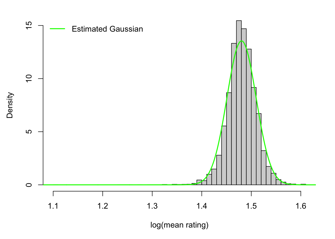
Using the estimated parameters \(\hat{\mu}^2_{\text{ML}}\) and \(\hat{\sigma}^2_{\text{ML}}\) the Gaussian distribution is fully defined and can be plotted onto the histogram of the data. See below in green:

Show code

x <- seq(-6, 0, .1)
data <- read.table("./data/mean_ratings.csv", header = T)
log_data <- log(data$mean)
hist(log_data, main = "", freq = F, ylim = c(0, .6)
)
lines(x, dnorm(x, mean(log_data), sqrt(1 / n * sum((
  log_data - mean(log_data)
) ^ 2))), lwd = 2, col = "green")

1.4 Method of Moments

The method of moments is one of the most classical approaches to parameter estimation. Although it is less commonly used today due to its limitations with complex models involving many parameters, we include it here for reasons of completeness.

1.4.1 Moments

Recall the definition of:

• the k-th empirical moment of a random variable \(X\) with \(n\) observations \(x_1,\ldots,x_n\): \[\hat{m}_k = \frac{1}{n}\sum_{i=1}^nx_i^k\]

• the k-th theoretical moment of this random variable, when assuming a distribution with parameter \(\theta\):

  \[m_{k}(\theta) = E_{\theta}(X^k)\]

1.4.2 Recipe

1. Link the moments of the random variables to the parameter(s) of the distribution: \[m_k(\thb) = \hat{m}_k, k = 1,\ldots,p\] (with \(p\) being the length of \(\thb\))
2. Solve for \(\theta\) (or all entries of \(\hat{\thb}\))
3. Obtain \(\hat{\theta}\) (or \(\hat{\thb}\))

1.4.3 Example: Bernoulli Distribution

Let’s look at the coin example from above. The parameter of interest here is \(p_H\):

First of all, we find the respective first moments from the Bernoulli distribution:

• first theoretical moment: \[m_1(p_H) = E_{p_H}(X) = 1\cdot P(X = H) + 0\cdot P(X = T) = p_H\]
• first empirical moment: \[m_1(x) = \frac{1}{n}\sum_{i=1}^nx_i = \frac{n_H}{n}\]

Next, we equate both moments: \[ m_1(p_H)\stackrel{!}{=}m_1(x) \\ \implies \hat{p}_{MOM} = \frac{n_H}{n} \]

1.5 Bias

Since estimators do not always perform equally well, we require different methods to assess their performance. One such method is called bias, which simply indicates whether the expectation of the estimator (\(E_{x|\theta}(\hat{\theta})\)) aligns with the parameter it is estimating (\(\theta\)).

The Bias of an estimator is defined as:

\[\mathrm{Bias}_{\theta}(\hat{\theta}) = \mathrm{E}_{\theta}(\hat{\theta})-\theta = \mathrm{E}_{\theta}(\hat{\theta}-\theta)\] An estimator \(\hat{\theta}\) is called unbiased, if its Bias is zero.

Is the estimator for \(\hat{\mu} = \bar{X}\) in the example with the Gaussian distribution unbiased?

Solution

In this case: \[ E_{\mu}(\bar{X}) = \frac{1}{n}\sum_{i=1}^nE_{\mu}(x_i) = \frac{1}{n}n\mu = \mu \] The bias is defined as: \[\mathrm{Bias}_{\mu}(\bar{X}) = \mathrm{E}_{\mu}(\hat{\mu})-\mu = \mathrm{E}_{\mu}(\hat{\mu}) = \mu - \mu = 0\] Hence, the estimator is unbiased!

1.6 Interactive Shiny App

You can play around with more random coin-flipping examples and see how we get more precise ML estimates for an increasing number of flips at our Maximum-Likelihood Shiny app.