Lecture 7 Boosting

7.1 Overview

Overview of this shiny with references to Sections comes here

7.2 Basic Principles

7.2.1 Intuition

Boosting is an additive learning method originally developed for classification problems. It can be adapted as an iterative estimation procedure for regression models.

Consider, for example, the linear model: \[y_i = \eta_i + \varepsilon_i = \xb_i^T\bb + \varepsilon_i, \quad i = 1,\dots,n.\] In some situations the ordinary least squares estimate is not optimal. In particular, when

the number $p$ of covariates large (especially when $p>n$)
the covariates are highly correlated
many covariates may not be related to the outcome at all

In Boosting, the coefficient estimate vector is initialized with $\hat{\bb} = 0$ and improved iteratively by adding new functions to reduce the residual error. In each iteration, a new regression on the residuals of the previous step is performed to obtain the least squares estimate $\hat{\boldsymbol{b}}$. The parameter vector $\hat{\bb}$ is then updated as a weighted sum of all past updates, with the weights controlled by the learning rate/step length $\nu$.

7.3 Algorithm

The following algorithm displays this basic idea:

Choose initial estimate $\hat\bb^{[0]}$, usually $\hat\bb^{[0]} = 0$, and number of total iterations $m_\text{stop}$. Set $m = 1$.
Compute the current residuals $\ub = \yb - \Xb\hat\bb^{[m-1]}$ and the least squares estimate $\hat{\boldsymbol{b}} = (\Xb^T\Xb)^{-1}\Xb^T\ub$. Update \[\hat\bb^{[m]} = \hat\bb^{[m-1]} + \nu\hat{\boldsymbol{b}}\] with $0<\nu<1$.
Set $m = m+1$.
Repeat steps 2 and 3 for $m_\text{stop}$ iterations.

Show R-Implementation

boost <- function(y, X, nu, mstop){
  beta <- rep(0, ncol(X))
  
  for(m in 1:mstop){
    u <- y - X%*%beta
    b <- solve(crossprod(X))%*%t(X)%*%u
    beta <- beta + nu*b
  }
  
  return(beta)
}

Note that:

From $\hat{\bb}^{[0]}$ the coefficient estimate iteratively converges to the maximum likelihood estimate, which in case of a Gaussian error coincides with the least squares estimate.
In each iteration only a small factor $\nu$ of the least squares estimate $\hat{\boldsymbol{b}}$ obtained from the current residuals $\ub$ is added. This factor $\nu$ is called step length or learning rate. $\nu$ is chosen rather small, usually $\nu = 0.1$ or $\nu = 0.01$.
In boosting terminology, the least squares estimate $\hat{\boldsymbol{b}}$ is called base learning procedure or base learner. The base learner provides the general fitting procedure and is then boosted by the boosting algorithm. There are many possible choices of base learners besides the one we use (e.g., penalized least squares, random effects, etc.), which we will not discuss here.
We will show in Section 7.5 that the algorithm can be stopped early leading to shrunken effect estimates compared to maximum likelihood. This effect shrinkage is also called regularization. The regularized estimation is useful since using either too many or using too few covariates may induce suboptimal predictions.

7.3.1 Interactive Illustration

Here comes the “basic principle”-tab from the corresponding shiny app.

7.4 Component-Wise Boosting

7.4.1 Algorithm

So far we updated all covariates combined in each iteration by $\hat{\boldsymbol{b}} = (\Xb^T\Xb)^{-1}\Xb^T\ub$. Now assume a univariate linear model $u_i = b_rx_{ir} + \varepsilon_{ir}$ for each covariate $\xb^r = (x_{1r},\dots,x_{nr})^T$, $r = 1,\dots,p$, i.e., we will equip each covariate $x_1,\dots,x_p$ with its own base learner.

Choose initial estimates $\hat\bb^{[0]}$, usually $\hat\bb^{[0]} = 0$, and number of total iterations $m_\text{stop}$. Set $m = 1$.
For every covariate $\xb^r$ the corresponding univariate model $u_i = b_rx_{ir} + \varepsilon_{ir}$ is fitted to the current residuals $\ub$: \[ \hat{b}_r = [(\xb^r)^T\xb^r]^{-1}(\xb^r)^T\ub = \frac{\sum_{i=1}^n (x_{ir} - \bar{x}_r)u_i}{\sum_{i=1}^n (x_{ir} - \bar{x}_r)^2}, \quad r = 1,\dots,p \]
Determine the optimal component \[ r^* = \underset{r = 1,\dots,p}\argmin \sum_{i=1}^n (u_i - x_{ir}\hat{b}_r)^2 \] leading to the largest reduction of the least squares criterion.
Update the coefficients by \[ \hat{\beta}_r^\text{new} = \begin{cases} \hat{\beta}_r^\text{old}, &\text{ if } r \neq r^*, \\ \hat{\beta}_r^\text{old} + \nu\hat{b}_{r^*}, &\text{ if } r = r^*. \end{cases} \]
Set $m = m+1$
Repeat steps 2 to 5 until $m = m_\text{stop}$.

Show R-Implementation

comp_boost <- function(y, X, nu, mstop){
  beta <- rep(0, ncol(X))
  
  for(m in 1:mstop){
    u <- y - X%*%beta
    b <- c()
    RSS <- c()
    for(r in 1:ncol(X)){
      b[r] <- solve(crossprod(X[,r]))%*%t(X[,r])%*%u
      RSS[r] <- sum((u - X[,r]*b[r])^2)
    }
    best <- which.min(RSS)
    beta[best] <- beta[best] + nu*b[best]
  }
  
  return(beta)
}

7.4.2 Comparison

Since we now do not optimize all components in the vector simultaneously, the convergence to the optimal solution follows a different trajectory compared to the regular method. We apply both approaches to finding the solution for the following regression equation: \[ y = 1 \cdot x_1 + 2 \cdot x_2 + \varepsilon \]

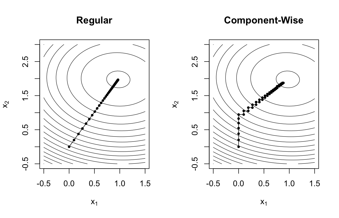
Using the R implementations from above the resulting optimization paths look like this:

Comparing the gradient paths shown in the plots, one observes that within 100 iterations the regular algorithm reaches the minimum of the loss function faster and along a more direct path. However, the regularized component-wise updates have several advantages when:

estimating models with a large number of covariates ($p \gg n$).
performing variable selection, since only the coefficients of the best-fitting covariates will be updated in each iteration.
estimating effects of correlated covariates.

7.4.3 Interactive Algorithm

Put “Demonstration of component-wise boosting” tab of the boosting shiny here (instead of slide 18). Remember to refer to Early Stopping Criteria (CV and AIC) in later sections.

7.5 Early Stopping

Usually, convergence to the OLS estimator is not desired. We thus do not let $m_{\text stop}$ run towards infinity but rather choose a small number of iterations to cause shrinkage of the estimated coefficients towards zero. This procedure is called early stopping of the algorithm which can be based on different pre-defined rules:

out-of-bag error
cross validation
bootstrapping
other rules like probing, information criteria, …

7.5.1 Out-Of-Bag Error

The out-of-bag error is one criterion to find the optimal number of iterations $m^*$ after which to stop the algorithm. First, split the data randomly into training $\Xb^\text{train}, \yb^\text{train}$ and test sample $\Xb^\text{test}, \yb^\text{test}$. Second, execute component-wise boosting on the training sample yielding $\hat{\bb}_\text{train}^{[m]}$, $m = 1,,m_ $. Last, find the optimal $m^*$ w.r.t. error on test data: \[\begin{align*} m^* &= \underset{m = 1,\dots,m_\text{stop}}\argmin \sum_{i=1}^{n^\text{test}} \left( y_i^\text{test} - \xb_i^\text{test}\hat{\bb}^{[m]} \right)^2 \\ &= \underset{m = 1,\dots,m_\text{stop}}\argmin \left\| \yb^\text{test} - \Xb^\text{test}\hat{\bb}_\text{train}^{[m]} \right\|^2 \end{align*}\]

To illustrate this graphically, we take the WeatherGermany dataset and filter it by the non-missing observations of June in Cuxhaven. Our variable of interest is the average temperature T which we regress on the amount of rainy days rain, the sunshine duration sun, the quality of data collection, the year and day. Calculating the out-of-bag error by using a 2:1 split for this arbitrarily chosen example, we find that the optimal test error is at $m=93$ iterations:

7.5.2 K-Fold Cross Validation

One problem that arises with the previous method is that splitting the data into training and test sample only once limits the information available or model fitting. We can gain a more robust computation of the out-of-bag error by using K-fold cross validation, which works in the following way:

Partition the data into $K$ fairly equal subsets $\Xb^k, \yb^k$, $k = 1,\dots,K$ to obtain a higher sample for calculating the criterion.
For each $k$ execute component-wise boosting on the training sample excluding the $k$-th subset: \[ \Xb^{-k} = \bigcup_{j\neq k} \Xb^j, \quad \yb^{-k} = \bigcup_{j\neq k} \yb^j \]. This yields $\hat{\bb}_{-k}^{[m]}$, $k = 1,\dots,K$ for $m = 1,\dots,m_\text{stop}$ iterations.
Find the optimal $m^*$ w.r.t. by evaluating the average test error over all subsets: \[ m^* = \underset{m = 1,\dots,m_\text{stop}}\argmin \frac1K \sum_{k = 1}^K \left\| \yb^k - \Xb^k\hat{\bb}_{-k}^{[m]} \right\|^2 \]

7.5.3 K-Fold Bootstrap

K-Fold Bootstrapping is similar to K-Fold Cross Validation, but instead of creating training sets by partitioning the data, each training set is obtained via bootstrapping:

For $k = 1,\dots,K$ obtain a training sample $\Xb^{-k}, \yb^{-k}$ by drawing $n$ entries with replacement from the original data $\Xb, \yb$.
Use the remaining observations not included in $\Xb^{-k}, \yb^{-k}$ as test data $\Xb^{k}, \yb^{k}$.
Fit the model $K$ times using the different single training samples yielding $\hat{\bb}_{-k}^{[m]}$.
For finding the optimal number of iterations $m^*$ as for $K$-fold cross validation: \[ m^* = \underset{m = 1,\dots,m_\text{stop}}\argmin \frac1K \sum_{k = 1}^K \left\| \yb^k - \Xb^k\hat{\bb}_{-k}^{[m]} \right\|^2 \]

With the very same example as in Section 7.5.1 we again provide a visualization that shows the optimal $m^*=116$ resulting from 25-fold bootstrapping:

7.5.4 Interactive Comparison of Methods

Here comes the “Variable Selection” Tab of the Gradient Boosting Shiny App.

7.6 Generic Component-Wise Boosting

The method discussed so far (linear model) is a special case of the more general component-wise gradient boosting. In the general case a loss function $\rho(\yb, \boldsymbol\eta)$ (usually chosen as the negative log-likelihood of the response variable) is minimized by fitting several base learners $\boldsymbol h_1,\dots,\boldsymbol h_p$ in a component-wise fashion to the negative gradient \[ \ub = - \frac{\partial\rho (y,\eta)}{\partial \eta} \] of the loss function $\rho$.

So far, in the linear model we used:

the loss function: \[ \rho = \sum_{i=1}^n\frac{1}{2}(y_i - \eta_i)^2 = \sum_{i=1}^n\frac{1}{2}(y_i - \xb_i^T \bb)^2 \] as the quadratic loss.
the negative gradient \[ \boldsymbol u = \frac{\partial \rho(\boldsymbol y, \boldsymbol \eta) }{\partial\eta} = \boldsymbol y - \boldsymbol \eta \] as the residuals.
the base learners \[ \boldsymbol h_r(\boldsymbol{x}_r) = \boldsymbol{b}_r \boldsymbol{x}_r \] as the linear effect of the r-th covariate.

In the linear model case, the loss function is defined as: \[ \rho = \sum_{i=1}^n\frac{1}{2}(y_i - \eta_i)^2 = \sum_{i=1}^n\frac{1}{2}(y_i - \xb_i^T \bb)^2 \] The following algorithm displays the generic way of component-wise Boosting:

Initialize predictor $\hat{\eta}^{[0]} \equiv 0$ and specify base learners $\boldsymbol h_1(\boldsymbol x_1),\dots,\boldsymbol h_p(\boldsymbol x_p)$. Set m = 1.
Compute the negative gradient \[ \ub^{[m]} = - \frac{\partial\rho (\boldsymbol y,\boldsymbol \eta)}{\partial \boldsymbol \eta} \bigg|_{\boldsymbol \eta = \hat{\boldsymbol \eta}^{[m-1]}} \] and fit it to each of the p base learners separately: \[ \ub^{[m]} \xrightarrow{\text{base learner}} \hat{\boldsymbol h}_r^{[m]}, \quad r = 1,\dots,p \] The resulting p regression fits yield p vectors of predicted values, where each vector is an estimate of $\boldsymbol u ^{[m]}$.
Select best fitting base learner according to the lowest total residual sum of squares (RSS): \[ r^* = \underset{r = 1,\dots,p}\argmin \sum_{i=1}^n \left(u_{i}^{[m]} - \hat{\boldsymbol h}_r^{[m]}(x_{ir})\right)^2 \]
Update corresponding \[\hat{\eta}^{[m]} = \hat{\eta}^{[m-1]} + \nu\hat{h}_{r^*}^{[m]}\]
Set $m = m+1$.
Repeat steps 2 to 4 until $m = m_\text{stop}$.
Find $m^*$ using one of the suitable criteria discussed above (cross validation, bootstrapping etc.). Computing the test error is then based on the chosen loss $\rho$: \[\begin{align} m^* &= \underset{m = 1,\dots,m_\text{stop}}\argmin \rho\left( \yb^\text{test}, \hat{\boldsymbol \eta}_\text{train}^{[m]} \right) \\ &= \underset{m = 1,\dots,m_\text{stop}}\argmin \frac1K \sum_{k = 1}^K \sum_{i = 1}^{n_k} \rho \left( y_{i,k}, \hat{\eta}_{i, -k}^{[m]} \right) \end{align}\]

Consequently, the component-wise boosting algorithm descends along the gradient of the empirical risk. The advantages mentioned in Section 7.4.2 regarding variable selection and model choice also apply here in the generic case. As only the best fitting base learner is selected for updating $\hat{\boldsymbol \eta}^{[m]}$, the more influential a base learner is, the higher its selection probability within the total number of iterations will be.

7.7 Boosting GLMs

7.7.1 Introduction

A Generalized Linear Model (GLM) connects the linear predictor $\eta = \xb^T\bb$ to the conditional mean \[\mu = \mathbb{E}[y|\xb] = h(\eta) \quad \text{or} \quad \eta = g(\mu), \] via the response function $h$ (or the link function $g = h^{-1}$). We can also use boosting here by choosing the negative log-likelihood as a boosting loss function: \[ \rho(y, \eta) = - \ell(y, \eta) \] Depending on the selected distribution from the exponential family the corresponding loss function looks as follows:

Gaussian: $\rho(y, \eta) = \frac12 (y - \eta)^2$; $u = y - \eta$
Binomial: $\rho(y, \eta) = -y\log p - (1 - y) \log (1 - p)$ with $p = e^\eta/(1 + e^\eta)$; $u = y - \frac{e^\eta}{1 + e^\eta}$
Poisson: Exercise!

7.7.2 Example

Considering the allbus dataset, we perform the same poisson regression as in Section 4.5:

library(mboost)
set.seed(666)
mod <- glmboost(tv_hour ~
                  worktime + sex + age + loginc,
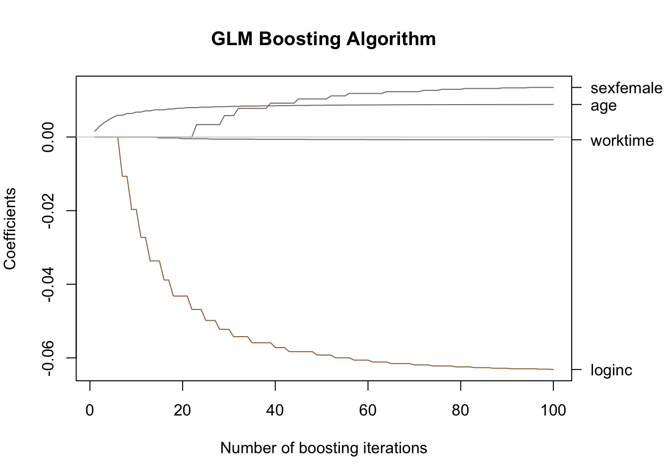
                data = allbus, family = Poisson())

In the following plot the coefficients’ progression when applying the boosting algorithm instead of MLE is shown:

plot(mod, ylim = range(coef(mod)[-1]),  off2int = T, main = "GLM Boosting Algorithm")

By applying cross-validated bootstrapping, we find that the optimal number of iterations equals 18:

set.seed(666)
boot <- cvrisk(mod)
mstop(boot)
plot(boot)

#> [1] 18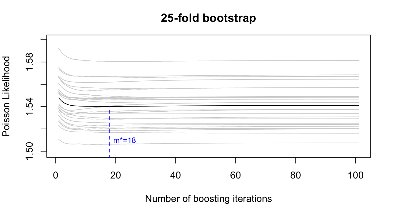

This provides a clear illustration of variable selection and regularization in action: the coefficients are noticeably smaller in absolute value compared to those reported in Section 4.5, and, moreover, the variable sex does not even appear in the output after the first 18 iterations:

coef(mod[mstop(boot)])
#>  (Intercept)     worktime          age       loginc 
#> -0.020932876 -0.000258631  0.007627423 -0.043203805 
#> attr(,"offset")
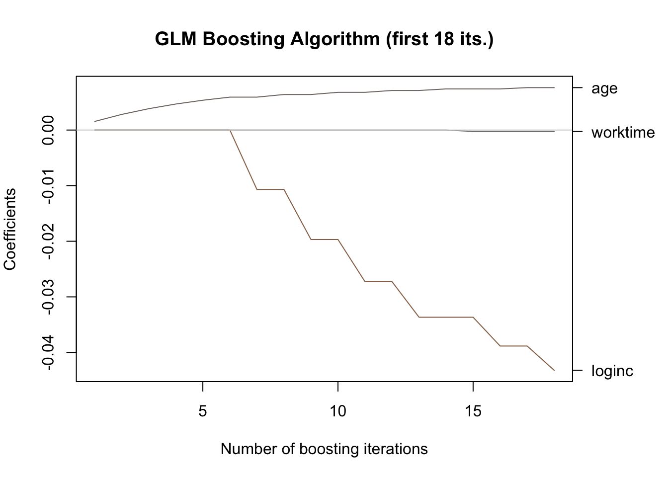
#> [1] 0.621546

Find below an excerpt showing only the first 18 iterations of the algorithm, which makes the relevant coefficient movements easier to evaluate:

plot(mod[mstop(boot)], ylim = range(coef(mod)[-1]),
     off2int = T, main = "GLM Boosting Algorithm (first 18 its.)")

6 Bayesian Modelling

8 Feed-Forward Neural Networks

Chair of Spatial Data Science and Statistical Learning

Introduction to Bayesian Inference and Statistical Learning