Lecture 2 Distributions
2.1 Overview
In this lecture, we will explore the distributions of discrete (Section 2.2.1) and continuous random variables (Section 2.2.2). To do so, we will introduce the most important distributions in Section 2.3, discuss their key properties, and examine the relationships between them.
2.2 Random Variables
A random variable is a variable that takes on numerical values determined by the outcome of a random process. We will start with the definition of distributions for the two different types of random variables.
2.2.1 Discrete Random Variables
A random variable is discrete if it can take on a finite or countably infinite number of distinct values. Examples include the number of heads when flipping a coin several times or the number of students in a classroom.
The probability mass function (PMF) \(f(x)\) for a discrete random variable \(X\) is defined as:\[f(x) = \left\{ \begin{array}{l} P(X = x_i) = p_i, \quad x = x_i \in \{x_1,x_2,\ldots,x_k,\ldots\}\\ 0, \qquad \qquad \qquad \quad \text{ else} \end{array} \right.\]
with finite or countable infinite possible values for \(x_1,x_2,\ldots, x_k,\ldots\), \(0\leq p_i \leq 1\) and \(\sum_{i\geq1}p_i = 1\).
The cumulative distribution function (CDF) \(F(x)\) for a discrete random variable \(X\) is defined as the sum of over all values of \(X\) that are less than or equal to \(x\):\[F(x) = P(X\leq x) = \sum_{i:x_i\leq x}f(x_i)\]
2.2.2 Continuous Random Variables
A random variable is continuous if it can take on an uncountable number of possible values within a range. Examples include the height of individuals oxfr the time it takes to complete a task.
The probability density function is defined as:\[ f(x) \geq 0, \quad \text{for all } x \in \mathbb{R}, \]
such that the probability of \(X\) falling within an interval \((a,b]\) is given by: \[P(a < X \leq b) = \int_a^b f(x) \,dx\] Additionally, the total probability must sum to one: \[\int_{-\infty}^{\infty} f(x) \,dx = 1\]
The cumulative distribution function \(F(x)\) for a continuous random variable \(X\) is defined as the integral of the PDF over all values less than or equal to \(x\):\[F(x) = P(X \leq x) = \int_{-\infty}^{x} f(t) \,dt\]
The CDF has the following properties:
- \(F(x)\) is continuous and monotonically increasing in \([0,1]\)
- \(F(-\infty) = \underset{x \rightarrow - \infty}{\lim} F(x) = 0\\ F(\infty) \; \; \, = \; \underset{x \rightarrow \infty}{\lim} \; F(x) = 1\)
- \(F^{\prime}= \frac{dF(x)}{dx} = f(x)\)
- \(P(a\leq X\leq b) = F(b) - F(a)\)
For discrete random variables, the probability of each possible outcome is explicitly defined and non-zero. In contrast, for continuous random variables, the probability of any specific value \(k\) is always zero \((P(X=k) = 0)\) because there are infinitely many possible values. Probabilities are meaningful only when defined over intervals, as determined by the density function \(f(x)\) or the cumulative distribution function \(F(x)\).
2.3 Distributions
In the following we will get to know different distributions. We will use the WeatherGermany dataset to illustrate them.
2.3.1 Weather Data
The WeatherGermany dataset provides weather observations from 681 weather stations across Germany, spanning the years 1936 to 2016. Each record describes a single observation made by one station at a specific point in time.
The following variables are contained:| Name | Description | Unit |
|---|---|---|
| id | identity of weather station location | |
| T | average air temperature 2 meters above the ground | degree Celsius |
| Tmin | minimum air temperature | degree Celsius |
| Tmax | maximum air temperature | degree Celsius |
| rain | amount of rain | millimeters/24h |
| sun | sunshine duration | hours |
| year | 1936 - 2016 | |
| month | 1 - 12 | |
| day | 1 - 31 | |
| alt | altitude | meter |
| lon | longitude | degree |
| lat | latitude | degree |
| name | location of weather station | |
| quality | quality of data collection |
Summary
summary(WeatherGermany)
#>       id                  T                Tmin
#>  Length:6949079     Min.   :-33.100   Min.   :-35.600
#>  Class :character   1st Qu.:  3.100   1st Qu.:  0.100
#>  Mode  :character   Median :  8.800   Median :  5.000
#>                     Mean   :  8.661   Mean   :  4.755
#>                     3rd Qu.: 14.500   3rd Qu.: 10.000
#>                     Max.   : 32.400   Max.   : 26.000
#>
#>       Tmax             rain             sun
#>  Min.   :-31.50   Min.   :  0.00   Min.   : 0.0
#>  1st Qu.:  6.10   1st Qu.:  0.00   1st Qu.: 0.2
#>  Median : 13.00   Median :  0.10   Median : 3.4
#>  Mean   : 12.81   Mean   :  2.22   Mean   : 4.4
#>  3rd Qu.: 19.50   3rd Qu.:  2.30   3rd Qu.: 7.6
#>  Max.   : 40.20   Max.   :312.00   Max.   :17.6
#>                   NA's   :156157   NA's   :3001007
#>       year          month             day
#>  Min.   :1936   Min.   : 1.000   Min.   : 1.00
#>  1st Qu.:1964   1st Qu.: 4.000   1st Qu.: 8.00
#>  Median :1982   Median : 7.000   Median :16.00
#>  Mean   :1981   Mean   : 6.535   Mean   :15.73
#>  3rd Qu.:2000   3rd Qu.:10.000   3rd Qu.:23.00
#>  Max.   :2016   Max.   :12.000   Max.   :31.00
#>
#>       alt               lon              lat
#>  Min.   :  -0.27   Min.   : 6.024   Min.   :47.40
#>  1st Qu.:  40.33   1st Qu.: 8.409   1st Qu.:49.29
#>  Median : 154.00   Median : 9.983   Median :51.13
#>  Mean   : 262.48   Mean   :10.141   Mean   :51.08
#>  3rd Qu.: 406.20   3rd Qu.:11.729   3rd Qu.:52.83
#>  Max.   :2964.00   Max.   :14.953   Max.   :54.91
#>
#>      name              quality            yday
#>  Length:6949079     Min.   : 3.000   Min.   :  1.0
#>  Class :character   1st Qu.: 5.000   1st Qu.: 92.0
#>  Mode  :character   Median : 5.000   Median :183.0
#>                     Mean   : 6.895   Mean   :183.3
#>                     3rd Qu.:10.000   3rd Qu.:275.0
#>                     Max.   :10.000   Max.   :365.0
#>
2.3.2 Gaussian Distribution
2.3.2.1 Definitions
The Gaussian distribution, also known as the normal distribution, is a continuous probability distribution defined by its mean (\(\mu\)) and variance (\(\sigma^2\)). It is widely used in statistics, as many natural phenomena and random variables follow this distribution.
The Gaussian distribution is important because it often models error terms in statistical models, and many estimators (like the maximum likelihood estimator) assume normality in the data. Additionally, the central limit theorem shows that the sum of many independent random variables tends to follow a Gaussian distribution which simplifies inference for large samples.
| Density | \(f(x|\mu,\sigma^2) = \frac{1}{\sqrt{2\pi\sigma^2}}\exp\left(-\frac{(x-\mu)^2}{2\sigma^2}\right)\) |
| Support | \(x \in \mathbb{R}\) |
| Notation & Parameters | \(X \sim \mathcal{N}(\mu,\sigma^2), \; \mu \in \mathbb{R}, \; \sigma > 0\) |
| Moments | \(\mathbb{E}(X) = \mu, \; \mathrm{Var}(x) = \sigma^2\) |
| Location Parameters | \(\mathrm{Mode}(X) = \mathrm{Median}(X) = \mu\) |
2.3.2.2 Example
The weather on the Brocken in March is one example for a random variable that can be modeled by the gaussian distribution.
Let’s have a look at the summary statistics for the minimum air temperature:
brocken <- WeatherGermany[WeatherGermany$name == "Brocken",]
br_mar <- brocken[brocken$month == 3,]$Tmin
summary(br_mar)
#>    Min. 1st Qu.  Median    Mean 3rd Qu.    Max.
#> -19.600  -7.000  -4.000  -4.086  -1.000  10.100
sd(br_mar)
#> [1] 4.423305
range(brocken$year)
#> [1] 1947 2016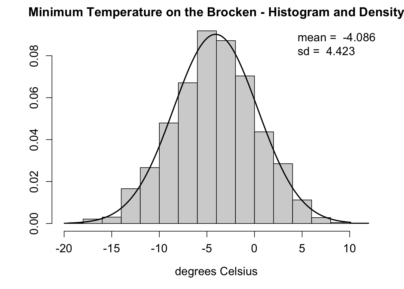
2.3.3 Chi-Squared Distribution
2.3.3.1 Definitions
The chi-squared distribution describes the sum of squared independent standard normal variables. It is parametrized by the degrees of freedom (\(k\)), which typically represents the number of summands. This distribution is always non-negative and skewed right, especially for smaller degrees of freedom. As the degrees of freedom increase, it becomes more symmetric and approaches a normal distribution. It is commonly used in hypothesis testing, calculating confidence intervals, and estimating variances.
| Density | \(f(x|k) = \frac{1}{2^{k/2}\Gamma(k/2)}x^{k/2 - 1}e^{-x/2}\\ \text{where} \;\Gamma(k/2) = \int_{0}^{\infty} x^{k/2-1}e^{-x}\: dx,\\\text{or} \; \Gamma(k/2) = (k/2 -1)! \; \text{when}\; k/2 \in \mathbb{N}\) |
| Support | \(x \in \mathbb{R}^+\) |
| Notation & Parameters | \(X \sim \chi^2(k), \; k \in \mathbb{N}\) (“degrees of freedom”) |
| Moments | \(\mathbb{E}(X) = k, \; \mathrm{Var}(x) = 2k\) |
| Location Parameters | \(\mathrm{Mode}(X) = \mathrm{max}(k-2,0)\\\mathrm{Median}(X) \approx k\Big(1 - \frac{2}{9k}\Big)^3\) |
2.3.3.2 Example 1: Temperature on Brocken
To construct chi-squared random variables, we standardize and square the minimum temperature on the Brocken. The degrees of freedom in this case are \(k = 1\).
br_mar_m <- mean(br_mar)
br_mar_sd <- sd(br_mar)

# Standardize
br_mar_std <- (br_mar - br_mar_m) / br_mar_sd

# Square
br_mar_chi <- br_mar_std^2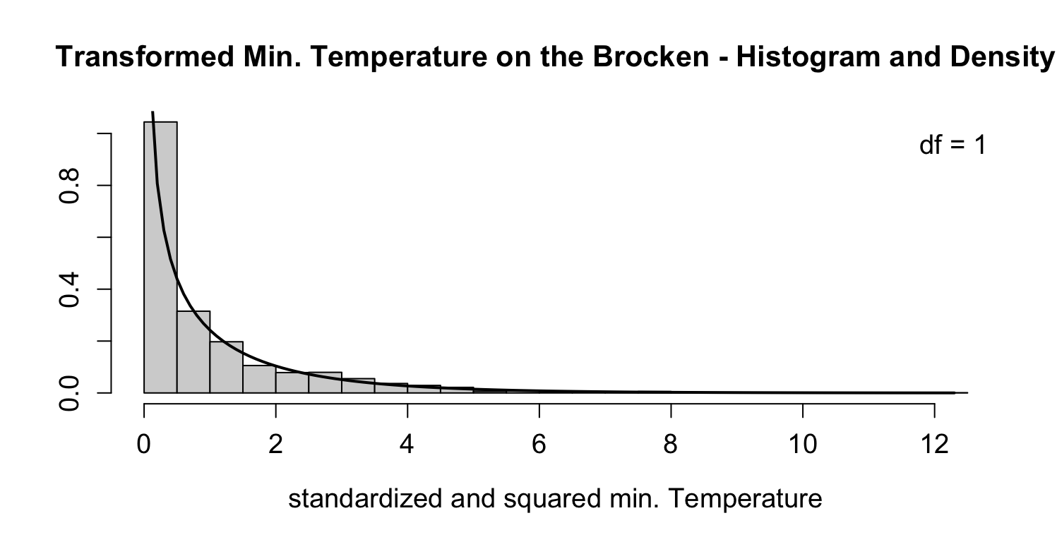
2.3.3.3 Example 2: Temperature in Arkona
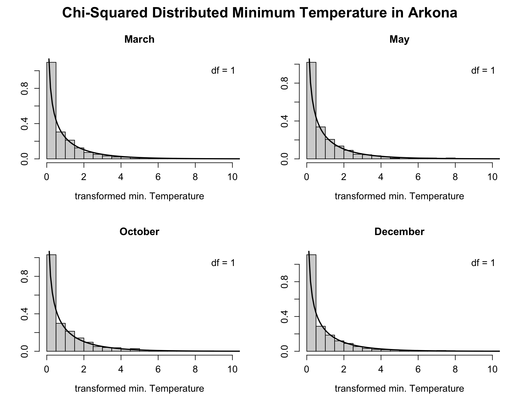
We can, however, also sum them up and again obtain a chi-square distributed random variable with four degrees of freedom (\(k = 4\)). The resulting density looks like this:
# Sum of the single Chi Squared distributions
chi_sum <- ark_mar_tmin_chi + ark_may_tmin_chi +
              ark_oct_tmin_chi + ark_dec_tmin_chi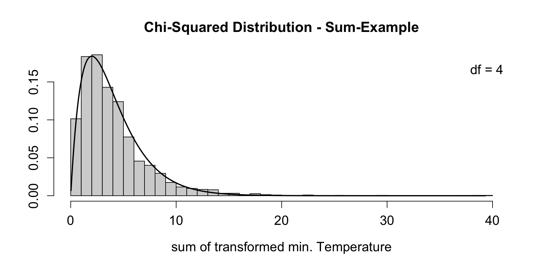
2.3.4 Poisson Distribution
2.3.4.1 Definitions
The Poisson distribution is used to model the number of events that occur within a fixed interval of time, space, or other continuous measure (e.g., distance or area), assuming these events happen independently and at a constant average rate. It is also called the distribution of the seldom events, as it is particularily suited for scenarios where events happen infrequently. When we have higher numbers of events we usually use an approximation via the Gaussian distribution.
| Probability Mass Function | \(f(x|\lambda) = \frac{\lambda^x}{x!} \mathrm{e}^{-\lambda}\) |
| Support | \(x \in \mathbb{N}_0\) |
| Notation & Parameters | \(X \sim \Po(\lambda), \; \lambda > 0\) |
| Moments | \(\mathbb{E}(X) = \mathrm{Var}(x) = \lambda\) |
| Location Parameters | \(\mathrm{Mode}(X) = \lambda, \, \lambda - 1\) \(\lambda - \ln 2 \leq \mathrm{Median}(X) < \lambda + \frac{1}{3}\) |
The fact that the Poisson distribution only has one parameter leads to quite a rigid form. The parameter \(\lambda\) is both, the expectation and the variance. This rather strict property is called equidispersion.
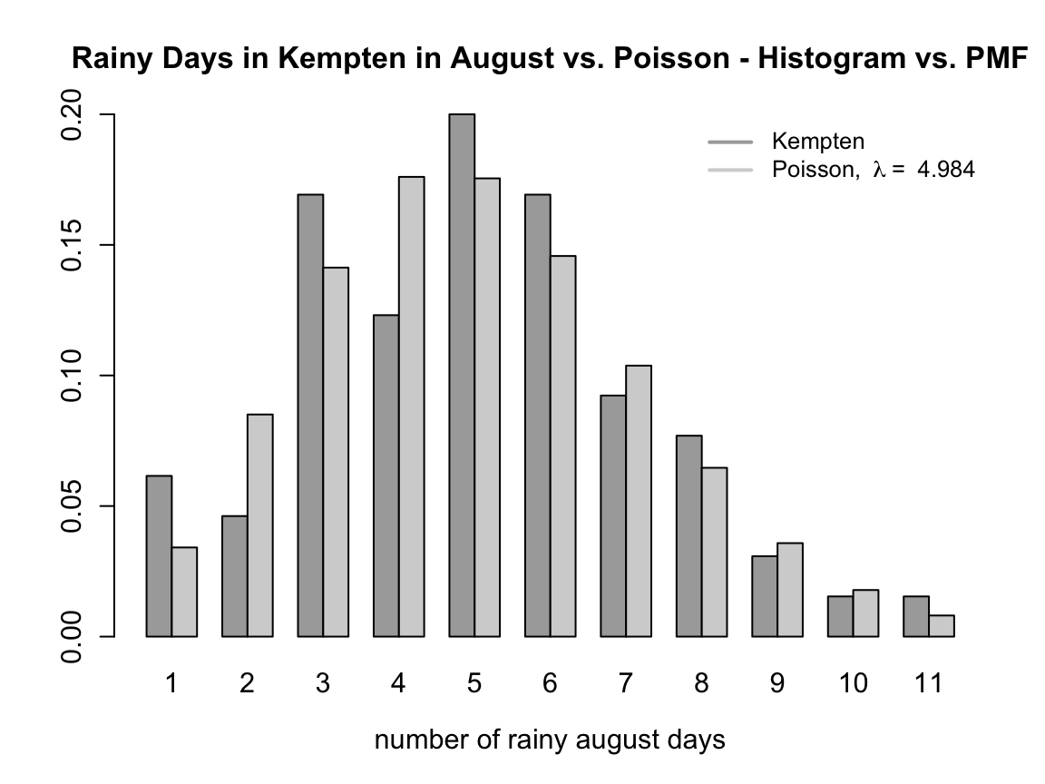
2.3.4.2 Example 1: Rain in Kempten
As an example for poisson distributed data we look at the rainy days in Kempten in August 1952 - 2016. We create the variable rainy by binarizing the continous information about the amount of rain using a specific treshold. The resulting summary statistics are as follows:
Kempten <- WeatherGermany[WeatherGermany$name == "Kempten",]
ke_aug <- Kempten[Kempten$month == 8,]
summary(rainy)
#>    Min. 1st Qu.  Median    Mean 3rd Qu.    Max.
#>   1.000   3.000   5.000   5.031   6.000  11.000
var(rainy)
#> [1] 4.936538
(lambda <- (mean(rainy) + var(rainy)) / 2)
#> [1] 4.983654
Using the average of the first two moments (mean and variance) we find an estimate for the rate \(\hat{\lambda}=4.984\).
Plotting the observed data against the theoretical Poisson distribution with the estimated parameter for \(\lambda\) we see that the poisson distribution might be a good guess. However, at the left-hand side of the mode there are some discrepancies.
2.3.4.3 Example 2: Rain in Braunlage
We now look at the rainy days in Braunlage in August (1936-2016). The following plot shows the distribution of the data and a theoretical poisson distribution using the mean of the data as an estimator for lambda (\(\hat{\lambda}=\overline{\text{rainy}}=6.079\)).
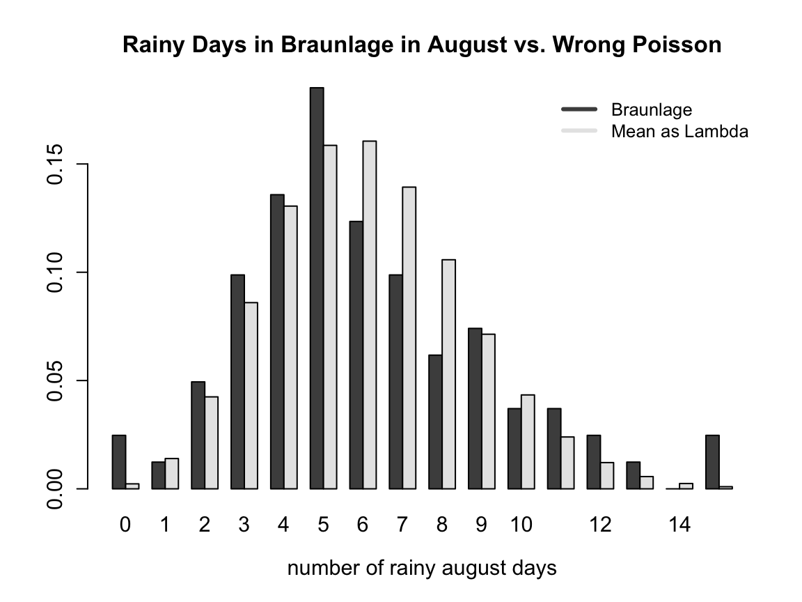
At first glance one can conclude that the data is poisson distributed. However, looking at the summary statistics we see that \(\bar{x} = 6.074 < \mathrm{Var}(x) = 9.744\) which is against the equidispersion assumption of the poisson distribution (underdispersion!). Hence, the poisson distribution is wrong here.
2.3.5 Gamma Distribution
2.3.5.1 Definitions
The Gamma distribution is a probability distribution that models positive continous random variables. This distribution will be mainly relevant for the Bayes part of this lecture. Be aware of the fact that there are many different kinds of parametrizations for this distribution.
| Density | \(f(x|\alpha,\beta) = \frac{\beta^\alpha}{\Gamma(\alpha)}x^{\alpha-1}\mathrm{e}^{-\beta x} \\ \text{where} \; \Gamma(\alpha) = \int_{0}^{\infty} x^{\alpha-1}e^{-x}\: dx, \\ \text{or} \;\Gamma(\alpha) = (\alpha -1)! \; \text{when}\; \alpha \in \mathbb{N}\) |
| Support | \(x \in \mathbb{R}^+\) |
| Notation & Parameters | \(X \sim \Gamma(\alpha,\beta), \; \alpha \in \mathbb{R}^+, \; \beta \in \mathbb{R}^+\) |
| Moments | \(\mathbb{E}(X) = \frac{\alpha}{\beta}, \; \mathrm{Var}(x) = \frac{\alpha}{\beta^2}\) |
| Location Parameters | \(\mathrm{Mode}(X) = \frac{\alpha - 1}{\beta} \: \text{for} \: \alpha \geq 1\) |
2.3.5.2 Example
The cumulative monthly rainfall (in millimeters) during autumn in Hamburg-Fuhlsbüttel (1936-2016) serves as an example for the Gamma distribution.
fuhl <- WeatherGermany[WeatherGermany$name == "Hamburg-Fuhlsbuettel",]
fuhl_autumn <- fuhl[which(fuhl$month == 9 |
                          fuhl$month == 10 |
                          fuhl$month == 11),]
In the following we calculate the summary statistics and calculate the Maximum-Likelihood Estimates for \(\alpha\) and \(\beta\).
#Object cum_rain_fuhl} contains cumulated rain in autumn in HH
summary(cum_rain_fuhl)
#>    Min. 1st Qu.  Median    Mean 3rd Qu.    Max.
#>    3.00   39.75   58.20   63.68   81.55  183.00
(alpha <- mean(cum_rain_fuhl)^2 / var(cum_rain_fuhl))
#> [1] 3.710252
(beta <- (var(cum_rain_fuhl) / mean(cum_rain_fuhl))^-1)
#> [1] 0.05826604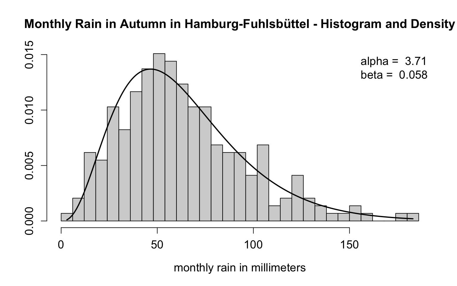
2.3.6 Inverse Gamma Distribution
2.3.6.1 Definitions
The inverse gamma distribution is a continuous probability distribution often used to model uncertainty in variance and scale parameters. It is defined for positive real values and parametrized by a shape parameter \(\alpha > 0\) and a scale parameter \(\beta > 0\). The inverse gamma is commonly applied in Bayesian statistics, especially as a prior for variance components. There are also many different parametrizations in literature.
| Support | \(x \in \mathbb{R}^+\) |
| Notation & Parameters | \(X \sim \Gamma^{-1}(\alpha, \beta), \; \alpha \in \mathbb{R}^+, \; \beta \in \mathbb{R}^+\) |
| Moments |
\(\mathbb{E}(X) = \frac{\beta}{\alpha - 1} \; \mathrm{for} \; \alpha > 1\) \(\mathrm{Var}(x) = \frac{\beta^2}{(\alpha-1)^2(\alpha-2)} \; \text{for} \; \alpha > 2\) |
| Location Parameters | \(\mathrm{Mode}(X) = \frac{\beta}{\alpha + 1}\) |
2.3.7 Beta Distribution
2.3.7.1 Definitions
The Beta distribution is a continuous probability distribution, commonly used to model proportions, probabilities, or random variables with bounded support. Two positive shape parameters and control the distribution’s shape. It is widely used in Bayesian statistics, particularly as a conjugate prior for binomial probabilities.
| Density | \(f(x|\alpha,\beta) = \frac{1}{B(\alpha, \beta)}x^{\alpha-1}(1-x)^{\beta-1} \\ \text{where} \; B(\alpha, \beta) = \frac{\Gamma(\alpha)\,\Gamma(\beta)}{\Gamma(\alpha + \beta)}\) |
| Support | \(x \in [0,1]\) |
| Notation & Parameters | \(X \sim Beta(\alpha, \beta), \; \alpha > 0, \; \beta > 0\) |
| Moments | \(\mathbb{E}(X) = \frac{\alpha}{\alpha+\beta}, \; \mathrm{Var}(x) = \frac{\alpha\beta}{(\alpha + \beta)^2(\alpha + \beta + 1)}\) |
| Location Parameters | \(\mathrm{Mode}(X) = \frac{\alpha - 1}{\alpha + \beta - 2} < \mathrm{Median}(X) < \mathbb{E}(X)\) |
2.3.7.2 Example
To construct an example that follows a beta distribution we calculate the proportion, prop, of days per year in Rosenheim which are warmer than 5°C (1950-2016). To obtain the estimated theoretical beta distribution we estimate the shape parameters using maximum likelihood.
Rosenheim <- WeatherGermany[WeatherGermany$name == "Rosenheim",]
m_prob <- mean(prob); v_prob <- var(prob)
(alpha <- m_prob * (((m_prob * (1 - m_prob)) / v_prob) - 1))
#> [1] 85.13278
(beta <- alpha / m_prob - alpha)
#> [1] 96.7454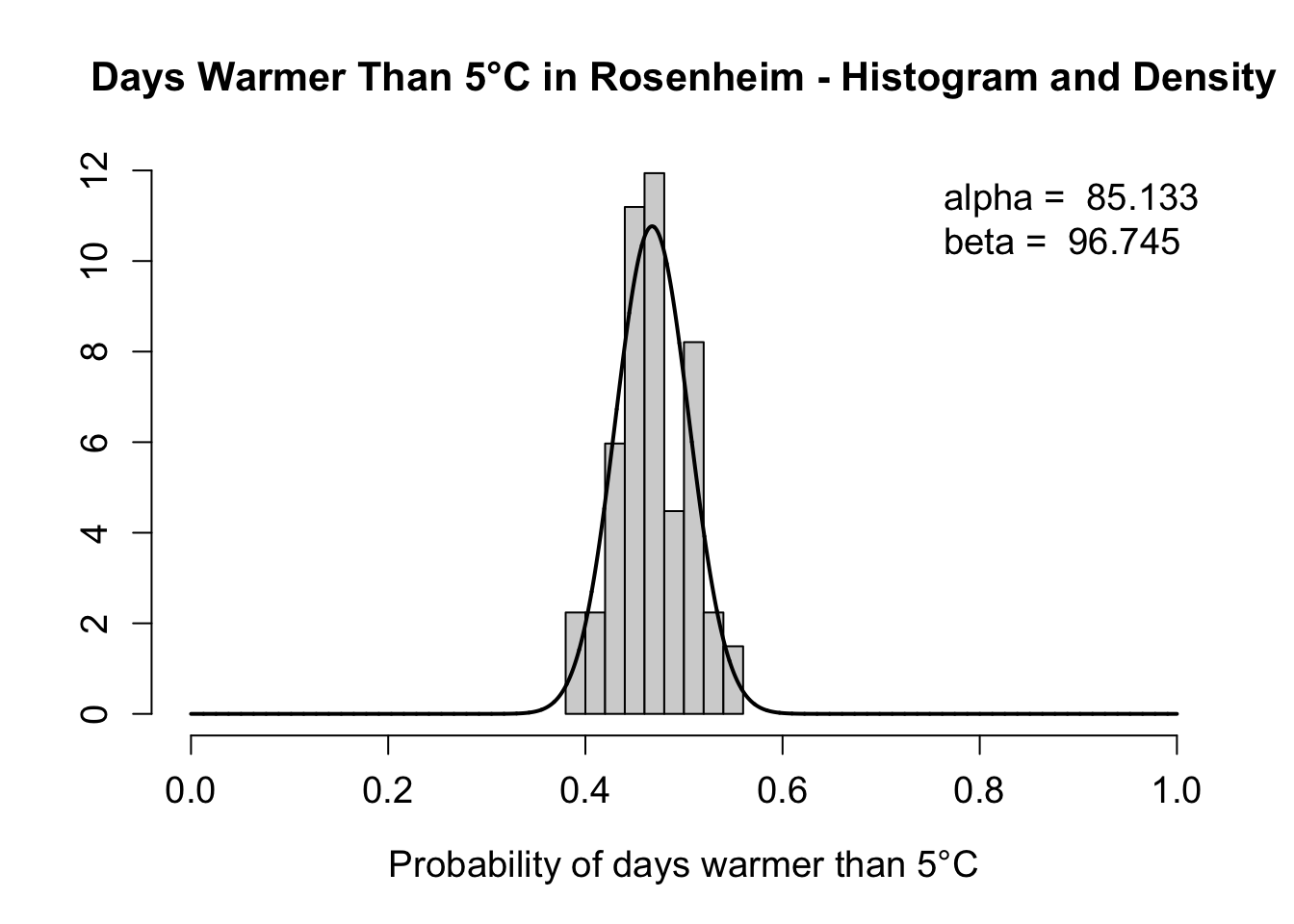
2.3.7.3 Interactive Distribution
You can play around with the sliders for the parameters \(\alpha\) and \(\beta\) to see how the distribution changes.
Hint: You can try out the following special cases:
- bell-shaped curve: \(\alpha = \beta = 5\)
- uniform distribution \(U(0,1)\): \(\alpha = \beta = 1\)
- bathtub curve: \(\alpha = \beta = 0.5\)
2.3.8 Exponential Distribution
2.3.8.1 Definitions
The exponential distribution is a continuous probability distribution commonly used to model the time between independent events occurring at a constant rate. It is defined for non-negative real numbers and parametrized by a rate parameter \(\lambda\) > 0, just like the Poisson distribution. The two distributions are closely related. Events, for which the waiting times are distributed with a Exponential distribution are themeselves distributed with a Poisson distribution. The exponential distribution is memoryless, meaning the probability of an event occurring in the future is independent of how much time has already elapsed.
| Density | \(f(x|\lambda) = \lambda e^{-\lambda x}\) |
| Support | \(x \in \mathbb{R}^+\) |
| Notation & Parameters | \(X \sim \Exp(\lambda), \; \lambda > 0\) |
| Moments | \(\mathbb{E}(X) = \frac{1}{\lambda}, \; \mathrm{Var}(x) = \frac{1}{\lambda^2}\) |
| Location Parameters | \(\mathrm{Mode}(X) = 0, \, \mathrm{Median}(X) = \frac{\ln 2}{\lambda}\) |
2.3.8.2 Example
We can model the waiting time between two rainy days in Bremen (1936-2016) via the exponential distribution. In the following we construct this variable, calculate the summary statistics and finally estimate the rate parameter using maximum likelihood:
Bremen <- WeatherGermany[WeatherGermany$name == "Bremen",]
bre_rain <- which(Bremen$rain > 10)
bre_wait <- diff(bre_rain)
summary(bre_wait)
#>    Min. 1st Qu.  Median    Mean 3rd Qu.    Max.
#>    1.00    4.00   13.00   22.64   30.00  219.00
bre_lam <- 1 / mean(bre_wait)
bre_lam
#> [1] 0.04416145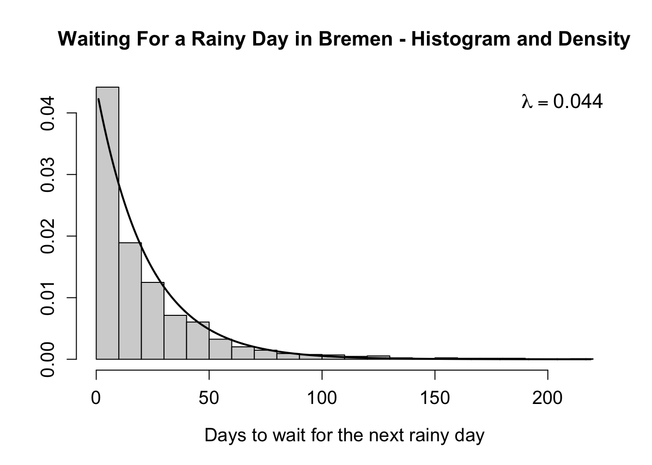
2.3.9 Binomial Distribution
2.3.9.1 Definitions
The binomial distribution is a discrete probability distribution that models the number of successes in a fixed number of independent Bernoulli trials, each with the same probability of success \(p\). The binomial distribution is commonly used to model binary outcomes, such as success/failure scenarios. It is one of the few distributions, which you could probably write down without too much theoretical knowledge, by just thinking about the nature of the random variable.
| Probability Mass Function | \(f(k|n, p) = \binom{n}{k} p^k (1-p)^{n-k}\) |
| Support | \(k \in \{0, 1, \dots, n\}\) (“number of successes”) |
| Notation & Parameters | \(X \sim B(n,p), \; n \in \mathbb{N}, \, p \in [0,1]\) |
| Moments | \(\mathbb{E}(X) = np, \; \mathrm{Var}(x) = np(1-p)\) |
| Location Parameters | \(\mathrm{Mode}(X) = \lfloor {(n+1)p} \rfloor\) |
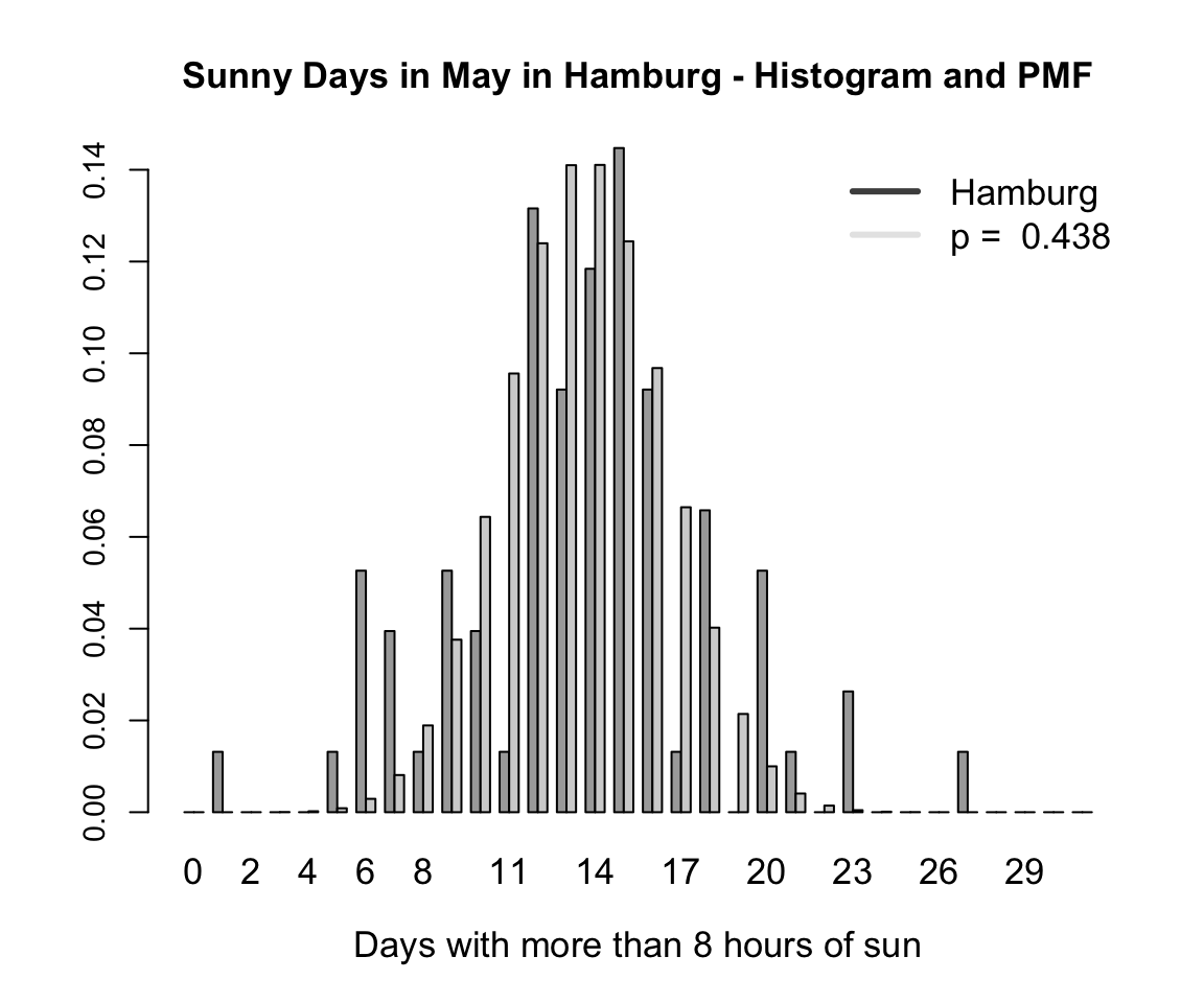
2.3.9.2 Example
As an example we look at the sunny days (>8h of sun) in May in Hamburg-Fuhlsbüttel (1936-2016) and create the variable hh_sun_may for this purpose. To obtain the theoretical binomial distribution, we take the fixed value \(n = 31\) and estimate the parameter \(p\) using maximum likelihood.
Hamburg <- WeatherGermany[WeatherGermany$name == "Hamburg-Fuhlsbuettel",]
hh_may <- Hamburg[Hamburg$month == 5,]
(p <- mean(hh_sun_may / 31))
#> [1] 0.4376061
We can now plot the discrete data as a histogram alongside the binomial distribution based on the estimated parameter for \(p\). Here, the y-axis represents the probability for each possible value of \(k\) (x-axis).
2.3.10 Multivariate Gaussian Distribution
2.3.10.1 Definitions
Finally, we turn to the Multivariate Gaussian distribution, which is particularly advantageous for multivariate continuous data. Notably, its marginal and conditional distributions are also Gaussian. The number of variables in the distribution is determined by \(k\), with the univariate Gaussian being a special case when \(k=1\).
| Density | \(f(x_1, \dots, x_k|\mub,\Sigb) =\frac{\exp\left(-\frac{1}{2}(\mathbf{x}-\mub)^T\Sigb^{-1}(\mathbf{x}-\mub)\right)}{\sqrt{(2\pi)^k|\Sigb|}}\) |
| Support | \(x \in \mub + \mathrm{span}(\Sigb) \subseteq \mathbb{R}^k\) |
| Notation & Parameters | \(X \sim \mathbf{\N}(\mub,\Sigb), \; \mub \in \mathbb{R}^k, \; \Sigb \in \mathbb{R}^{k \times k}\) |
| Moments | \(\mathbb{E}(X) = \mub, \; \mathrm{Var}(x) = \Sigb\) |
| Location Parameters | \(\mathrm{Mode}(X) = \mub\) |
2.3.10.2 Example
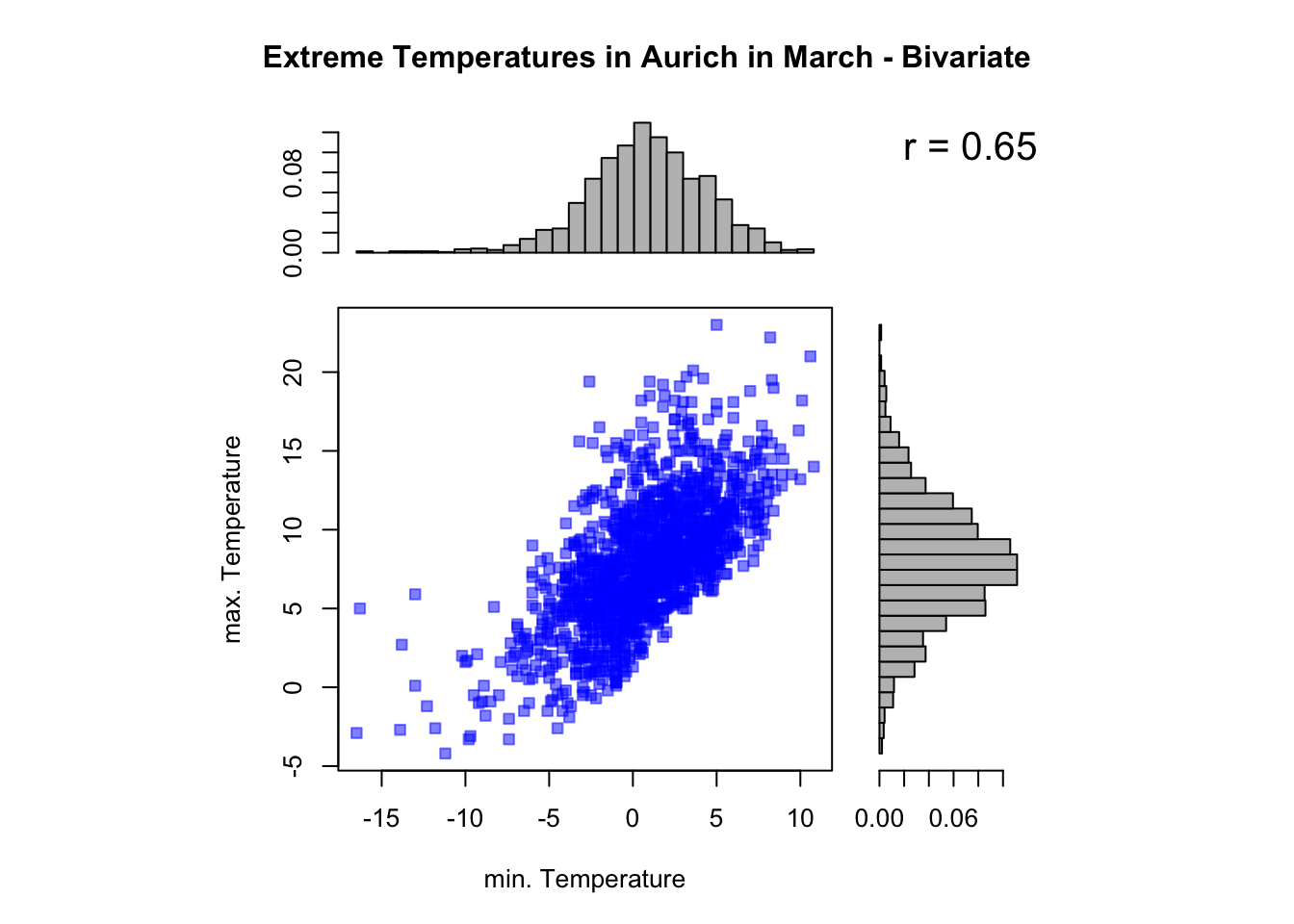
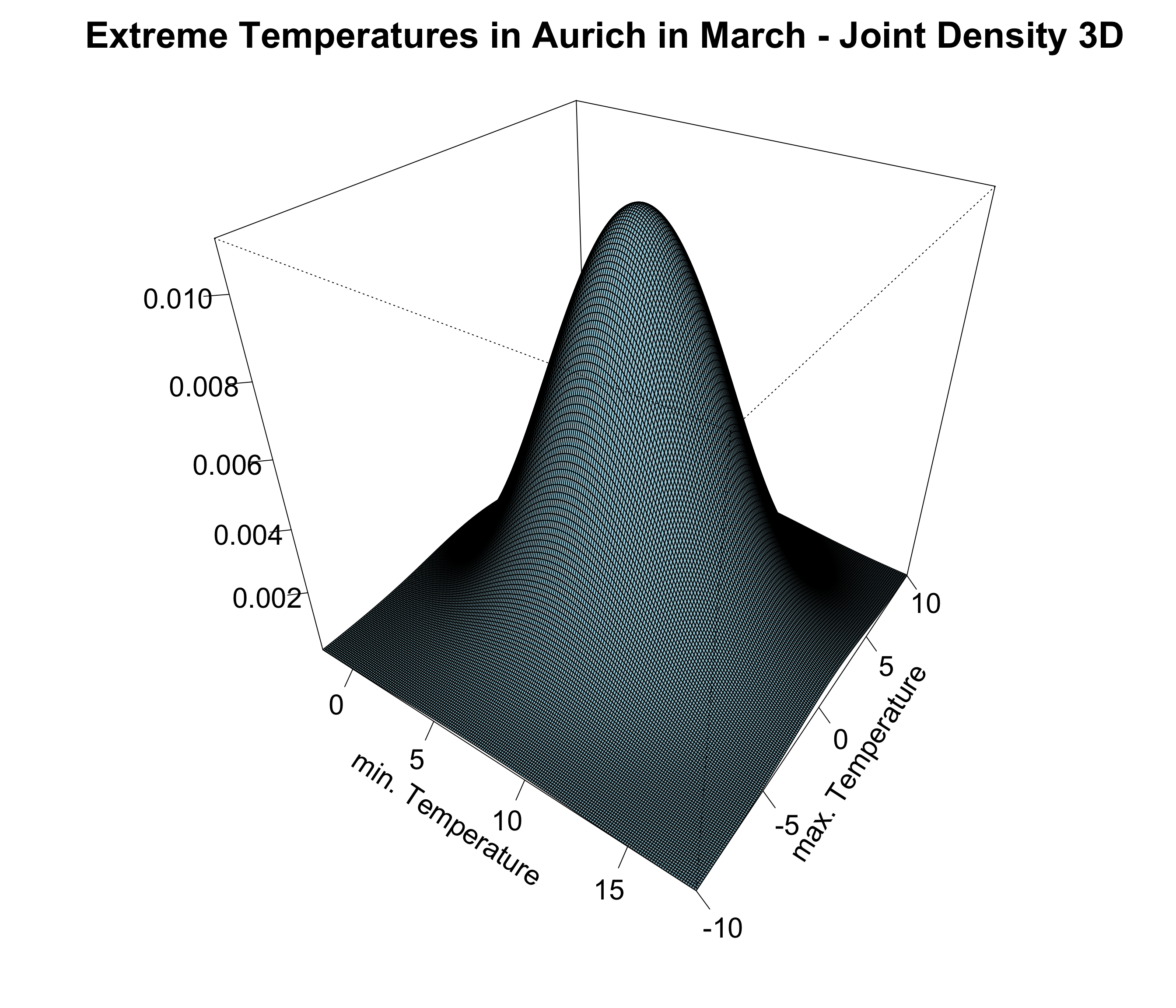
As an example we look at the joint distribution of extreme temperatures (min and max) in Aurich in March (1959-2006), which are both individually gaussian distributed.
To estimate the mean parameter, we compute the individual means. For the variance-covariance matrix, we estimate the variances along the diagonal and the covariances in the off-diagonal elements. It is important to note that this matrix is quadratic, symmetric, and positive semi-definite.
Aur <- WeatherGermany[WeatherGermany$name == "Aurich",]
aur_mar <- Aur[Aur$month == 3,]

mu1 <- mean(aur_mar$Tmax); mu2 <- mean(aur_mar$Tmin)
mu1; mu2
#> [1] 7.936895
#> [1] 0.834543

sig1 <- var(aur_mar$Tmax); sig2 <- var(aur_mar$Tmin)
rho <- cor(aur_mar$Tmax, aur_mar$Tmin)
(SIGMA <- matrix(c(sig1, rho, rho, sig2), ncol = 2))
#>            [,1]       [,2]
#> [1,] 16.0170844  0.6476699
#> [2,]  0.6476699 12.7118120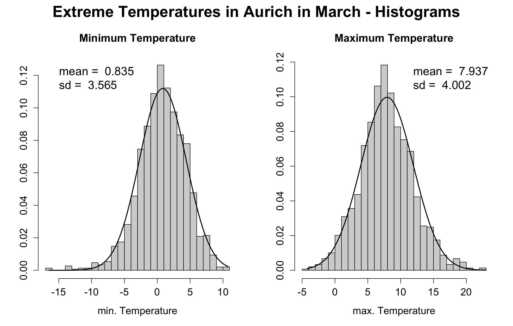
In the next step, we examine the bivariate scatter plot to determine if there is a correlation between the minimum and maximum temperatures. The plot reveals a strong positive correlation with a correlation coefficient of \(r = 0.65\). The histograms on the sides illustrate the individual marginal distributions of the temperatures.
2.3.11 Relations Between Distributions
As already mentioned, most of the distributions are closely related since they all come from the same family (“Exponential Family”).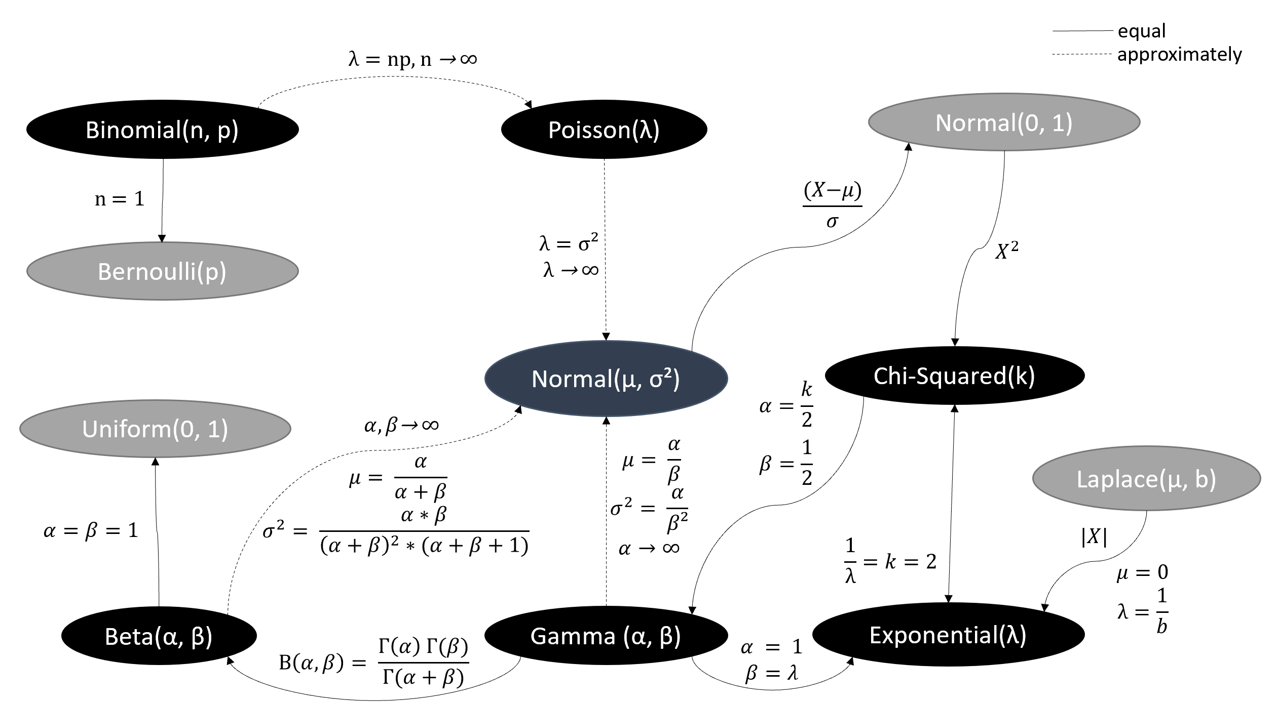
Figure 2.1: Based on Univariate Distribution Relationships by Leemis and McQueston, p. 45 - 53, in The American Statistician, 2008.
Feel free to check these relationships in the following app:
Click here for the full version of the univariate distribution shiny app and here for the full version of the multivariate distribution shiny app.