Chapter 5 Laboratorio 3 - Aula 8
5.1 Inibina B como marcador
library(caret)
library(MASS)

#GET("Dados/inibina.xls", write_disk(tf <- tempfile(fileext = ".xls")))

#dados01_cen01 = read_excel("Dados/inibina.xls", sheet = 1)
inibina <- read_excel("Dados/inibina.xls")
str(inibina)
## tibble [32 × 4] (S3: tbl_df/tbl/data.frame)
## $ ident : num [1:32] 1 2 3 4 5 6 7 8 9 10 ...
## $ resposta: chr [1:32] "positiva" "positiva" "positiva" "positiva" ...
## $ inibpre : num [1:32] 54 159.1 98.3 85.3 127.9 ...
## $ inibpos : num [1:32] 65.9 281.1 305.4 434.4 229.3 ...nrow(inibina)## [1] 32sum()## [1] 0inibina$difinib = inibina$inibpos - inibina$inibpre
inibina$resposta = as.factor(inibina$resposta)
plot(inibina$difinib ~ inibina$resposta, ylim = c(0, 400))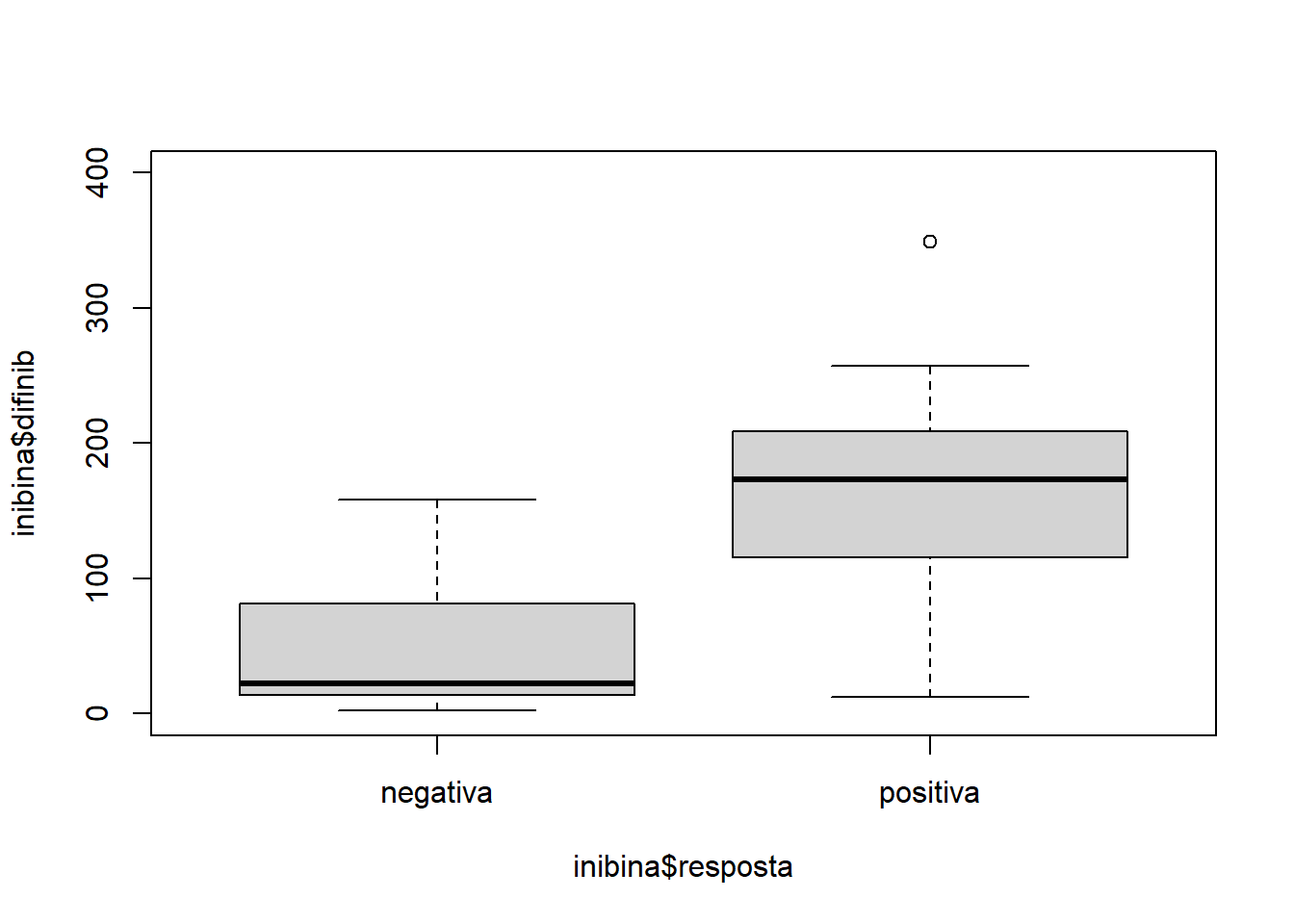
print(inibina, n = 32)## # A tibble: 32 × 5
## ident resposta inibpre inibpos difinib
## <dbl> <fct> <dbl> <dbl> <dbl>
## 1 1 positiva 54.0 65.9 11.9
## 2 2 positiva 159. 281. 122.
## 3 3 positiva 98.3 305. 207.
## 4 4 positiva 85.3 434. 349.
## 5 5 positiva 128. 229. 101.
## 6 6 positiva 144. 354. 210.
## 7 7 positiva 111. 254. 143.
## 8 8 positiva 47.5 199. 152.
## 9 9 positiva 123. 328. 205.
## 10 10 positiva 166. 339. 174.
## 11 11 positiva 145. 377. 232.
## 12 12 positiva 186. 1055. 869.
## 13 13 positiva 149. 354. 204.
## 14 14 positiva 33.3 100. 66.8
## 15 15 positiva 182. 358. 177.
## 16 16 positiva 58.4 168. 110.
## 17 17 positiva 128. 228. 100.
## 18 18 positiva 153. 312. 159.
## 19 19 positiva 149. 406. 257.
## 20 20 negativa 81 201. 120.
## 21 21 negativa 24.7 45.2 20.4
## 22 22 negativa 3.02 6.03 3.01
## 23 23 negativa 4.27 17.8 13.5
## 24 24 negativa 99.3 128. 28.6
## 25 25 negativa 108. 129. 21.1
## 26 26 negativa 7.36 21.3 13.9
## 27 27 negativa 161. 320. 158.
## 28 28 negativa 184. 311. 127.
## 29 29 negativa 23.1 45.6 22.5
## 30 30 negativa 111. 192. 81.0
## 31 31 negativa 106. 131. 24.8
## 32 32 negativa 3.98 6.46 2.48# Hmisc::describe(inibina)
summary(inibina)## ident resposta inibpre inibpos
## Min. : 1.00 negativa:13 Min. : 3.02 Min. : 6.03
## 1st Qu.: 8.75 positiva:19 1st Qu.: 52.40 1st Qu.: 120.97
## Median :16.50 Median :109.44 Median : 228.89
## Mean :16.50 Mean :100.53 Mean : 240.80
## 3rd Qu.:24.25 3rd Qu.:148.93 3rd Qu.: 330.77
## Max. :32.00 Max. :186.38 Max. :1055.19
## difinib
## Min. : 2.48
## 1st Qu.: 24.22
## Median :121.18
## Mean :140.27
## 3rd Qu.:183.77
## Max. :868.81sd(inibina$difinib)## [1] 159.22175.1.1 Generalized Linear Models
modLogist01 = glm(resposta ~ difinib, family = binomial, data = inibina)
summary(modLogist01)
##
## Call:
## glm(formula = resposta ~ difinib, family = binomial, data = inibina)
##
## Deviance Residuals:
## Min 1Q Median 3Q Max
## -1.9770 -0.5594 0.1890 0.5589 2.0631
##
## Coefficients:
## Estimate Std. Error z value Pr(>|z|)
## (Intercept) -2.310455 0.947438 -2.439 0.01474 *
## difinib 0.025965 0.008561 3.033 0.00242 **
## ---
## Signif. codes: 0 '***' 0.001 '**' 0.01 '*' 0.05 '.' 0.1 ' ' 1
##
## (Dispersion parameter for binomial family taken to be 1)
##
## Null deviance: 43.230 on 31 degrees of freedom
## Residual deviance: 24.758 on 30 degrees of freedom
## AIC: 28.758
##
## Number of Fisher Scoring iterations: 6predito = predict.glm(modLogist01, type = "response")
classPred = ifelse(predito>0.5, "positiva", "negativa")
classPred = as.factor(classPred)
confusionMatrix(classPred, inibina$resposta, positive = "positiva")## Confusion Matrix and Statistics
##
## Reference
## Prediction negativa positiva
## negativa 10 2
## positiva 3 17
##
## Accuracy : 0.8438
## 95% CI : (0.6721, 0.9472)
## No Information Rate : 0.5938
## P-Value [Acc > NIR] : 0.002273
##
## Kappa : 0.6721
##
## Mcnemar's Test P-Value : 1.000000
##
## Sensitivity : 0.8947
## Specificity : 0.7692
## Pos Pred Value : 0.8500
## Neg Pred Value : 0.8333
## Prevalence : 0.5938
## Detection Rate : 0.5312
## Detection Prevalence : 0.6250
## Balanced Accuracy : 0.8320
##
## 'Positive' Class : positiva
## 5.1.2 LDA - Fisher
modFisher01 = lda(resposta ~ difinib, data = inibina, prior = c(0.5, 0.5))
predito = predict(modFisher01)
classPred = predito$class
confusionMatrix(classPred, inibina$resposta, positive = "positiva")
## Confusion Matrix and Statistics
##
## Reference
## Prediction negativa positiva
## negativa 11 6
## positiva 2 13
##
## Accuracy : 0.75
## 95% CI : (0.566, 0.8854)
## No Information Rate : 0.5938
## P-Value [Acc > NIR] : 0.04978
##
## Kappa : 0.5058
##
## Mcnemar's Test P-Value : 0.28884
##
## Sensitivity : 0.6842
## Specificity : 0.8462
## Pos Pred Value : 0.8667
## Neg Pred Value : 0.6471
## Prevalence : 0.5938
## Detection Rate : 0.4062
## Detection Prevalence : 0.4688
## Balanced Accuracy : 0.7652
##
## 'Positive' Class : positiva
## 5.1.3 BAYES
inibina$resposta## [1] positiva positiva positiva positiva positiva positiva positiva positiva
## [9] positiva positiva positiva positiva positiva positiva positiva positiva
## [17] positiva positiva positiva negativa negativa negativa negativa negativa
## [25] negativa negativa negativa negativa negativa negativa negativa negativa
## Levels: negativa positivamodBayes01 = lda(resposta ~ difinib, data = inibina, prior = c(0.65, 0.35))
predito = predict(modBayes01)
classPred = predito$class
# table(classPred)
confusionMatrix(classPred, inibina$resposta, positive = "positiva")## Confusion Matrix and Statistics
##
## Reference
## Prediction negativa positiva
## negativa 13 13
## positiva 0 6
##
## Accuracy : 0.5938
## 95% CI : (0.4064, 0.763)
## No Information Rate : 0.5938
## P-Value [Acc > NIR] : 0.5755484
##
## Kappa : 0.2727
##
## Mcnemar's Test P-Value : 0.0008741
##
## Sensitivity : 0.3158
## Specificity : 1.0000
## Pos Pred Value : 1.0000
## Neg Pred Value : 0.5000
## Prevalence : 0.5938
## Detection Rate : 0.1875
## Detection Prevalence : 0.1875
## Balanced Accuracy : 0.6579
##
## 'Positive' Class : positiva
## # inibina$resposta
# modBayes01 = lda(resposta ~ difinib, data = inibina, prior = c(0.35, 0.65))
# predito = predict(modBayes01)
# classPred = predito$class
# confusionMatrix(classPred, inibina$resposta, positive = "positiva")
print(inibina, n = 32)## # A tibble: 32 × 5
## ident resposta inibpre inibpos difinib
## <dbl> <fct> <dbl> <dbl> <dbl>
## 1 1 positiva 54.0 65.9 11.9
## 2 2 positiva 159. 281. 122.
## 3 3 positiva 98.3 305. 207.
## 4 4 positiva 85.3 434. 349.
## 5 5 positiva 128. 229. 101.
## 6 6 positiva 144. 354. 210.
## 7 7 positiva 111. 254. 143.
## 8 8 positiva 47.5 199. 152.
## 9 9 positiva 123. 328. 205.
## 10 10 positiva 166. 339. 174.
## 11 11 positiva 145. 377. 232.
## 12 12 positiva 186. 1055. 869.
## 13 13 positiva 149. 354. 204.
## 14 14 positiva 33.3 100. 66.8
## 15 15 positiva 182. 358. 177.
## 16 16 positiva 58.4 168. 110.
## 17 17 positiva 128. 228. 100.
## 18 18 positiva 153. 312. 159.
## 19 19 positiva 149. 406. 257.
## 20 20 negativa 81 201. 120.
## 21 21 negativa 24.7 45.2 20.4
## 22 22 negativa 3.02 6.03 3.01
## 23 23 negativa 4.27 17.8 13.5
## 24 24 negativa 99.3 128. 28.6
## 25 25 negativa 108. 129. 21.1
## 26 26 negativa 7.36 21.3 13.9
## 27 27 negativa 161. 320. 158.
## 28 28 negativa 184. 311. 127.
## 29 29 negativa 23.1 45.6 22.5
## 30 30 negativa 111. 192. 81.0
## 31 31 negativa 106. 131. 24.8
## 32 32 negativa 3.98 6.46 2.48modKnn1_01 = knn3(resposta ~ difinib, data = inibina, k = 1)
predito = predict(modKnn1_01, inibina, type = "class")
confusionMatrix(predito, inibina$resposta, positive = "positiva")## Confusion Matrix and Statistics
##
## Reference
## Prediction negativa positiva
## negativa 13 0
## positiva 0 19
##
## Accuracy : 1
## 95% CI : (0.8911, 1)
## No Information Rate : 0.5938
## P-Value [Acc > NIR] : 5.693e-08
##
## Kappa : 1
##
## Mcnemar's Test P-Value : NA
##
## Sensitivity : 1.0000
## Specificity : 1.0000
## Pos Pred Value : 1.0000
## Neg Pred Value : 1.0000
## Prevalence : 0.5938
## Detection Rate : 0.5938
## Detection Prevalence : 0.5938
## Balanced Accuracy : 1.0000
##
## 'Positive' Class : positiva
## modKnn3_01 = knn3(resposta ~ difinib, data = inibina, k = 3)
predito = predict(modKnn3_01, inibina, type = "class")
confusionMatrix(predito, inibina$resposta, positive = "positiva")## Confusion Matrix and Statistics
##
## Reference
## Prediction negativa positiva
## negativa 11 2
## positiva 2 17
##
## Accuracy : 0.875
## 95% CI : (0.7101, 0.9649)
## No Information Rate : 0.5938
## P-Value [Acc > NIR] : 0.0005536
##
## Kappa : 0.7409
##
## Mcnemar's Test P-Value : 1.0000000
##
## Sensitivity : 0.8947
## Specificity : 0.8462
## Pos Pred Value : 0.8947
## Neg Pred Value : 0.8462
## Prevalence : 0.5938
## Detection Rate : 0.5312
## Detection Prevalence : 0.5938
## Balanced Accuracy : 0.8704
##
## 'Positive' Class : positiva
## modKnn5_01 = knn3(resposta ~ difinib, data = inibina, k = 5)
predito = predict(modKnn5_01, inibina, type = "class")
confusionMatrix(predito, inibina$resposta, positive = "positiva")## Confusion Matrix and Statistics
##
## Reference
## Prediction negativa positiva
## negativa 9 1
## positiva 4 18
##
## Accuracy : 0.8438
## 95% CI : (0.6721, 0.9472)
## No Information Rate : 0.5938
## P-Value [Acc > NIR] : 0.002273
##
## Kappa : 0.6639
##
## Mcnemar's Test P-Value : 0.371093
##
## Sensitivity : 0.9474
## Specificity : 0.6923
## Pos Pred Value : 0.8182
## Neg Pred Value : 0.9000
## Prevalence : 0.5938
## Detection Rate : 0.5625
## Detection Prevalence : 0.6875
## Balanced Accuracy : 0.8198
##
## 'Positive' Class : positiva
## library(e1071)
modNaiveBayes01 = naiveBayes(resposta ~ difinib, data = inibina)
predito = predict(modNaiveBayes01, inibina)
confusionMatrix(predito, inibina$resposta, positive = "positiva")## Confusion Matrix and Statistics
##
## Reference
## Prediction negativa positiva
## negativa 11 5
## positiva 2 14
##
## Accuracy : 0.7812
## 95% CI : (0.6003, 0.9072)
## No Information Rate : 0.5938
## P-Value [Acc > NIR] : 0.02102
##
## Kappa : 0.5625
##
## Mcnemar's Test P-Value : 0.44969
##
## Sensitivity : 0.7368
## Specificity : 0.8462
## Pos Pred Value : 0.8750
## Neg Pred Value : 0.6875
## Prevalence : 0.5938
## Detection Rate : 0.4375
## Detection Prevalence : 0.5000
## Balanced Accuracy : 0.7915
##
## 'Positive' Class : positiva
## library(rpart)
library(rpart.plot)5.1.4 Decision Tree
modArvDec01 = rpart(resposta ~ difinib, data = inibina)
prp(modArvDec01, faclen=0, #use full names for factor labels
extra=1, #display number of observations for each terminal node
roundint=F, #don't round to integers in output
digits=5)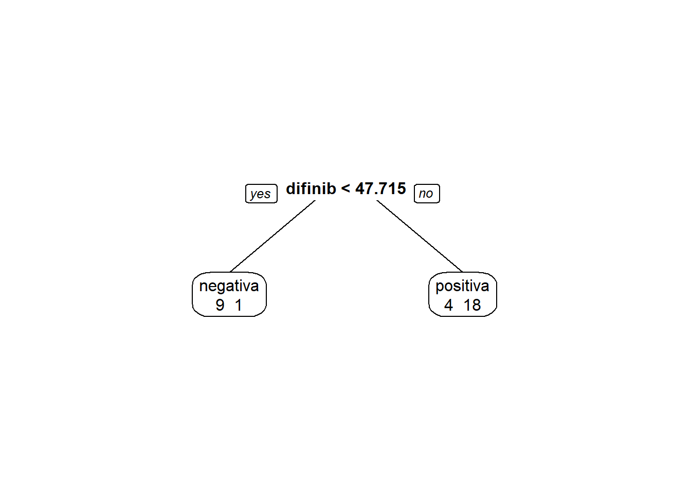
predito = predict(modArvDec01, type = "class")
confusionMatrix(predito, inibina$resposta, positive = "positiva")## Confusion Matrix and Statistics
##
## Reference
## Prediction negativa positiva
## negativa 9 1
## positiva 4 18
##
## Accuracy : 0.8438
## 95% CI : (0.6721, 0.9472)
## No Information Rate : 0.5938
## P-Value [Acc > NIR] : 0.002273
##
## Kappa : 0.6639
##
## Mcnemar's Test P-Value : 0.371093
##
## Sensitivity : 0.9474
## Specificity : 0.6923
## Pos Pred Value : 0.8182
## Neg Pred Value : 0.9000
## Prevalence : 0.5938
## Detection Rate : 0.5625
## Detection Prevalence : 0.6875
## Balanced Accuracy : 0.8198
##
## 'Positive' Class : positiva
## x = 1:32
plot(inibina$difinib ~x, col = inibina$resposta)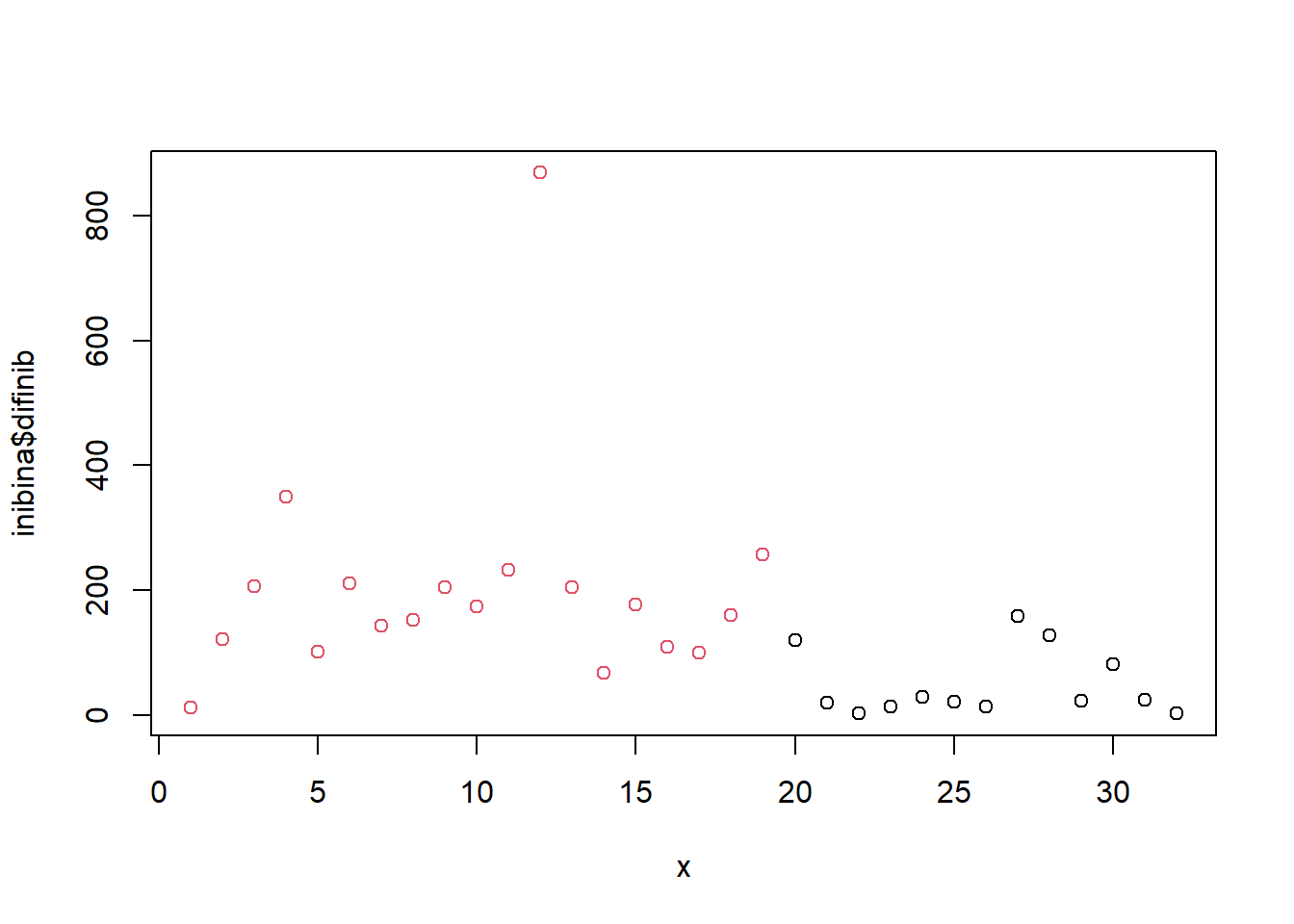
5.1.5 SVM
modSVM01 = svm(resposta ~ difinib, data = inibina, kernel = "linear")
predito = predict(modSVM01, type = "class")
confusionMatrix(predito, inibina$resposta, positive = "positiva")## Confusion Matrix and Statistics
##
## Reference
## Prediction negativa positiva
## negativa 10 2
## positiva 3 17
##
## Accuracy : 0.8438
## 95% CI : (0.6721, 0.9472)
## No Information Rate : 0.5938
## P-Value [Acc > NIR] : 0.002273
##
## Kappa : 0.6721
##
## Mcnemar's Test P-Value : 1.000000
##
## Sensitivity : 0.8947
## Specificity : 0.7692
## Pos Pred Value : 0.8500
## Neg Pred Value : 0.8333
## Prevalence : 0.5938
## Detection Rate : 0.5312
## Detection Prevalence : 0.6250
## Balanced Accuracy : 0.8320
##
## 'Positive' Class : positiva
## 5.1.6 Neural Network
library(neuralnet)
modRedNeural01 = neuralnet(resposta ~ difinib, data = inibina, hidden = c(2,4,3))
plot(modRedNeural01)
ypred = neuralnet::compute(modRedNeural01, inibina)
yhat = ypred$net.result
round(yhat)## [,1] [,2]
## [1,] 1 0
## [2,] 0 1
## [3,] 0 1
## [4,] 0 1
## [5,] 0 1
## [6,] 0 1
## [7,] 0 1
## [8,] 0 1
## [9,] 0 1
## [10,] 0 1
## [11,] 0 1
## [12,] 0 1
## [13,] 0 1
## [14,] 0 1
## [15,] 0 1
## [16,] 0 1
## [17,] 0 1
## [18,] 0 1
## [19,] 0 1
## [20,] 0 1
## [21,] 1 0
## [22,] 1 0
## [23,] 1 0
## [24,] 1 0
## [25,] 1 0
## [26,] 1 0
## [27,] 0 1
## [28,] 0 1
## [29,] 1 0
## [30,] 0 1
## [31,] 1 0
## [32,] 1 0yhat=data.frame("yhat"=ifelse(max.col(yhat[ ,1:2])==1, "negativa", "positiva"))
cm = confusionMatrix(inibina$resposta, as.factor(yhat$yhat))
print(cm)## Confusion Matrix and Statistics
##
## Reference
## Prediction negativa positiva
## negativa 9 4
## positiva 1 18
##
## Accuracy : 0.8438
## 95% CI : (0.6721, 0.9472)
## No Information Rate : 0.6875
## P-Value [Acc > NIR] : 0.03739
##
## Kappa : 0.6639
##
## Mcnemar's Test P-Value : 0.37109
##
## Sensitivity : 0.9000
## Specificity : 0.8182
## Pos Pred Value : 0.6923
## Neg Pred Value : 0.9474
## Prevalence : 0.3125
## Detection Rate : 0.2812
## Detection Prevalence : 0.4062
## Balanced Accuracy : 0.8591
##
## 'Positive' Class : negativa
## library(caret)
trControl <- trainControl(method = "LOOCV")
fit <- train(resposta ~ difinib, method = "glm", data = inibina,
trControl = trControl, metric = "Accuracy")
fit <- train(resposta ~ difinib, method = "lda", data = inibina, prior = c(0.5, 0.5),
trControl = trControl, metric = "Accuracy")
fit <- train(resposta ~ difinib, method = "lda", data = inibina, prior = c(0.65, 0.35),
trControl = trControl, metric = "Accuracy")
fit <- train(resposta ~ difinib, method = "knn", data = inibina,
tuneGrid = expand.grid(k = 1:5),
trControl = trControl, metric = "Accuracy")
# fit <- train(resposta ~ difinib, method = "svm", data = inibina,
# trControl = trControl, metric = "Accuracy")
# fit <- train(formula = resposta ~ difinib, method = "neuralnet", data = data.frame(inibina), hidden = c(2,3),
# linear.output = T,
# trControl = trControl, metric = "Accuracy")
totalAcerto = 0
for (i in 1:nrow(inibina)){
treino = inibina[-i,]
teste = inibina[i,]
modelo = svm(resposta ~ difinib, data = treino)
predito = predict(modelo, newdata = teste, type = "class")
if(predito == teste$resposta[1]) totalAcerto = totalAcerto+1
}
iris = tibble(iris)
irisS = iris[,1:4]
d <- dist(irisS, method = "maximum")
grup = hclust(d, method = "ward.D")
plot(grup, cex = 0.6)
groups <- cutree(grup, k=3)
table(groups, iris$Species)##
## groups setosa versicolor virginica
## 1 50 0 0
## 2 0 50 15
## 3 0 0 35rect.hclust(grup, k=3, border="red")
library(factoextra)
library(ggpubr)
km1 = kmeans(irisS, 4)
p1 = fviz_cluster(km1, data=irisS,
palette = c("#2E9FDF", "#FC4E07", "#E7B800", "#E7B700"),
star.plot=FALSE,
# repel=TRUE,
ggtheme=theme_bw())
p1
groups = km1$cluster
table(groups, iris$Species)##
## groups setosa versicolor virginica
## 1 17 0 0
## 2 0 2 36
## 3 33 0 0
## 4 0 48 14#remotes::Install_github("ExabytE1337/Lori")
datasets::iris## Sepal.Length Sepal.Width Petal.Length Petal.Width Species
## 1 5.1 3.5 1.4 0.2 setosa
## 2 4.9 3.0 1.4 0.2 setosa
## 3 4.7 3.2 1.3 0.2 setosa
## 4 4.6 3.1 1.5 0.2 setosa
## 5 5.0 3.6 1.4 0.2 setosa
## 6 5.4 3.9 1.7 0.4 setosa
## 7 4.6 3.4 1.4 0.3 setosa
## 8 5.0 3.4 1.5 0.2 setosa
## 9 4.4 2.9 1.4 0.2 setosa
## 10 4.9 3.1 1.5 0.1 setosa
## 11 5.4 3.7 1.5 0.2 setosa
## 12 4.8 3.4 1.6 0.2 setosa
## 13 4.8 3.0 1.4 0.1 setosa
## 14 4.3 3.0 1.1 0.1 setosa
## 15 5.8 4.0 1.2 0.2 setosa
## 16 5.7 4.4 1.5 0.4 setosa
## 17 5.4 3.9 1.3 0.4 setosa
## 18 5.1 3.5 1.4 0.3 setosa
## 19 5.7 3.8 1.7 0.3 setosa
## 20 5.1 3.8 1.5 0.3 setosa
## 21 5.4 3.4 1.7 0.2 setosa
## 22 5.1 3.7 1.5 0.4 setosa
## 23 4.6 3.6 1.0 0.2 setosa
## 24 5.1 3.3 1.7 0.5 setosa
## 25 4.8 3.4 1.9 0.2 setosa
## 26 5.0 3.0 1.6 0.2 setosa
## 27 5.0 3.4 1.6 0.4 setosa
## 28 5.2 3.5 1.5 0.2 setosa
## 29 5.2 3.4 1.4 0.2 setosa
## 30 4.7 3.2 1.6 0.2 setosa
## 31 4.8 3.1 1.6 0.2 setosa
## 32 5.4 3.4 1.5 0.4 setosa
## 33 5.2 4.1 1.5 0.1 setosa
## 34 5.5 4.2 1.4 0.2 setosa
## 35 4.9 3.1 1.5 0.2 setosa
## 36 5.0 3.2 1.2 0.2 setosa
## 37 5.5 3.5 1.3 0.2 setosa
## 38 4.9 3.6 1.4 0.1 setosa
## 39 4.4 3.0 1.3 0.2 setosa
## 40 5.1 3.4 1.5 0.2 setosa
## 41 5.0 3.5 1.3 0.3 setosa
## 42 4.5 2.3 1.3 0.3 setosa
## 43 4.4 3.2 1.3 0.2 setosa
## 44 5.0 3.5 1.6 0.6 setosa
## 45 5.1 3.8 1.9 0.4 setosa
## 46 4.8 3.0 1.4 0.3 setosa
## 47 5.1 3.8 1.6 0.2 setosa
## 48 4.6 3.2 1.4 0.2 setosa
## 49 5.3 3.7 1.5 0.2 setosa
## 50 5.0 3.3 1.4 0.2 setosa
## 51 7.0 3.2 4.7 1.4 versicolor
## 52 6.4 3.2 4.5 1.5 versicolor
## 53 6.9 3.1 4.9 1.5 versicolor
## 54 5.5 2.3 4.0 1.3 versicolor
## 55 6.5 2.8 4.6 1.5 versicolor
## 56 5.7 2.8 4.5 1.3 versicolor
## 57 6.3 3.3 4.7 1.6 versicolor
## 58 4.9 2.4 3.3 1.0 versicolor
## 59 6.6 2.9 4.6 1.3 versicolor
## 60 5.2 2.7 3.9 1.4 versicolor
## 61 5.0 2.0 3.5 1.0 versicolor
## 62 5.9 3.0 4.2 1.5 versicolor
## 63 6.0 2.2 4.0 1.0 versicolor
## 64 6.1 2.9 4.7 1.4 versicolor
## 65 5.6 2.9 3.6 1.3 versicolor
## 66 6.7 3.1 4.4 1.4 versicolor
## 67 5.6 3.0 4.5 1.5 versicolor
## 68 5.8 2.7 4.1 1.0 versicolor
## 69 6.2 2.2 4.5 1.5 versicolor
## 70 5.6 2.5 3.9 1.1 versicolor
## 71 5.9 3.2 4.8 1.8 versicolor
## 72 6.1 2.8 4.0 1.3 versicolor
## 73 6.3 2.5 4.9 1.5 versicolor
## 74 6.1 2.8 4.7 1.2 versicolor
## 75 6.4 2.9 4.3 1.3 versicolor
## 76 6.6 3.0 4.4 1.4 versicolor
## 77 6.8 2.8 4.8 1.4 versicolor
## 78 6.7 3.0 5.0 1.7 versicolor
## 79 6.0 2.9 4.5 1.5 versicolor
## 80 5.7 2.6 3.5 1.0 versicolor
## 81 5.5 2.4 3.8 1.1 versicolor
## 82 5.5 2.4 3.7 1.0 versicolor
## 83 5.8 2.7 3.9 1.2 versicolor
## 84 6.0 2.7 5.1 1.6 versicolor
## 85 5.4 3.0 4.5 1.5 versicolor
## 86 6.0 3.4 4.5 1.6 versicolor
## 87 6.7 3.1 4.7 1.5 versicolor
## 88 6.3 2.3 4.4 1.3 versicolor
## 89 5.6 3.0 4.1 1.3 versicolor
## 90 5.5 2.5 4.0 1.3 versicolor
## 91 5.5 2.6 4.4 1.2 versicolor
## 92 6.1 3.0 4.6 1.4 versicolor
## 93 5.8 2.6 4.0 1.2 versicolor
## 94 5.0 2.3 3.3 1.0 versicolor
## 95 5.6 2.7 4.2 1.3 versicolor
## 96 5.7 3.0 4.2 1.2 versicolor
## 97 5.7 2.9 4.2 1.3 versicolor
## 98 6.2 2.9 4.3 1.3 versicolor
## 99 5.1 2.5 3.0 1.1 versicolor
## 100 5.7 2.8 4.1 1.3 versicolor
## 101 6.3 3.3 6.0 2.5 virginica
## 102 5.8 2.7 5.1 1.9 virginica
## 103 7.1 3.0 5.9 2.1 virginica
## 104 6.3 2.9 5.6 1.8 virginica
## 105 6.5 3.0 5.8 2.2 virginica
## 106 7.6 3.0 6.6 2.1 virginica
## 107 4.9 2.5 4.5 1.7 virginica
## 108 7.3 2.9 6.3 1.8 virginica
## 109 6.7 2.5 5.8 1.8 virginica
## 110 7.2 3.6 6.1 2.5 virginica
## 111 6.5 3.2 5.1 2.0 virginica
## 112 6.4 2.7 5.3 1.9 virginica
## 113 6.8 3.0 5.5 2.1 virginica
## 114 5.7 2.5 5.0 2.0 virginica
## 115 5.8 2.8 5.1 2.4 virginica
## 116 6.4 3.2 5.3 2.3 virginica
## 117 6.5 3.0 5.5 1.8 virginica
## 118 7.7 3.8 6.7 2.2 virginica
## 119 7.7 2.6 6.9 2.3 virginica
## 120 6.0 2.2 5.0 1.5 virginica
## 121 6.9 3.2 5.7 2.3 virginica
## 122 5.6 2.8 4.9 2.0 virginica
## 123 7.7 2.8 6.7 2.0 virginica
## 124 6.3 2.7 4.9 1.8 virginica
## 125 6.7 3.3 5.7 2.1 virginica
## 126 7.2 3.2 6.0 1.8 virginica
## 127 6.2 2.8 4.8 1.8 virginica
## 128 6.1 3.0 4.9 1.8 virginica
## 129 6.4 2.8 5.6 2.1 virginica
## 130 7.2 3.0 5.8 1.6 virginica
## 131 7.4 2.8 6.1 1.9 virginica
## 132 7.9 3.8 6.4 2.0 virginica
## 133 6.4 2.8 5.6 2.2 virginica
## 134 6.3 2.8 5.1 1.5 virginica
## 135 6.1 2.6 5.6 1.4 virginica
## 136 7.7 3.0 6.1 2.3 virginica
## 137 6.3 3.4 5.6 2.4 virginica
## 138 6.4 3.1 5.5 1.8 virginica
## 139 6.0 3.0 4.8 1.8 virginica
## 140 6.9 3.1 5.4 2.1 virginica
## 141 6.7 3.1 5.6 2.4 virginica
## 142 6.9 3.1 5.1 2.3 virginica
## 143 5.8 2.7 5.1 1.9 virginica
## 144 6.8 3.2 5.9 2.3 virginica
## 145 6.7 3.3 5.7 2.5 virginica
## 146 6.7 3.0 5.2 2.3 virginica
## 147 6.3 2.5 5.0 1.9 virginica
## 148 6.5 3.0 5.2 2.0 virginica
## 149 6.2 3.4 5.4 2.3 virginica
## 150 5.9 3.0 5.1 1.8 virginicairis = tibble(iris)
unique(iris$Species)## [1] setosa versicolor virginica
## Levels: setosa versicolor virginicaplot(Sepal.Length ~ Petal.Length, data = iris, col = Species)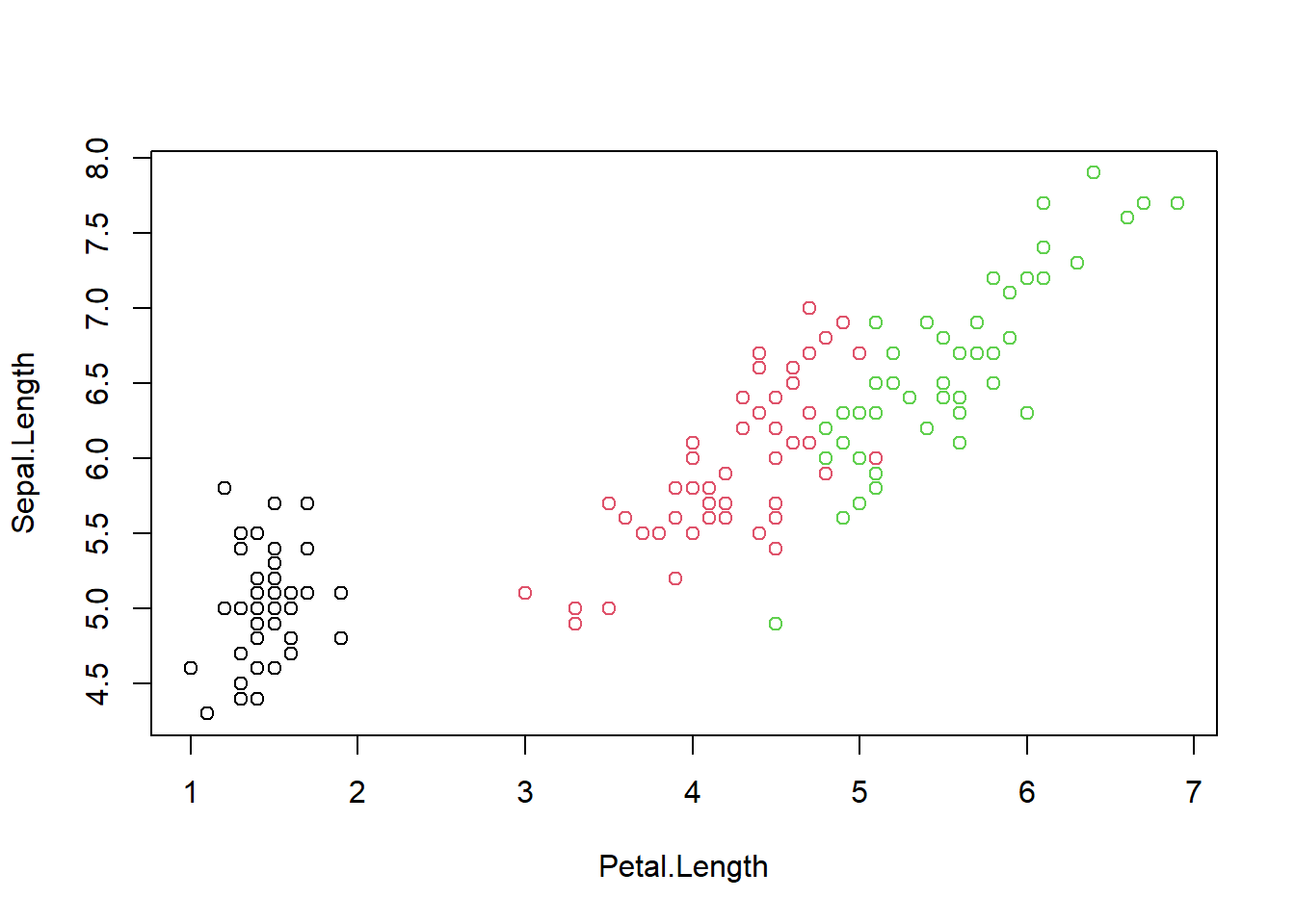
dadosSub = filter(iris, Species == "setosa" | Species == "versicolor")
dadosSub$Species = factor(as.character(dadosSub$Species))
modelRegLog01 = glm(Species ~ ., data = dadosSub, family = binomial)
summary(modelRegLog01)##
## Call:
## glm(formula = Species ~ ., family = binomial, data = dadosSub)
##
## Deviance Residuals:
## Min 1Q Median 3Q Max
## -1.681e-05 -2.110e-08 0.000e+00 2.110e-08 2.006e-05
##
## Coefficients:
## Estimate Std. Error z value Pr(>|z|)
## (Intercept) 6.556 601950.324 0 1
## Sepal.Length -9.879 194223.245 0 1
## Sepal.Width -7.418 92924.451 0 1
## Petal.Length 19.054 144515.981 0 1
## Petal.Width 25.033 216058.936 0 1
##
## (Dispersion parameter for binomial family taken to be 1)
##
## Null deviance: 1.3863e+02 on 99 degrees of freedom
## Residual deviance: 1.3166e-09 on 95 degrees of freedom
## AIC: 10
##
## Number of Fisher Scoring iterations: 25pred = predict.glm(modelRegLog01, type = "response")
predClass = ifelse(pred<0.5, "setosa", "versicolor")
confusionMatrix(as.factor(predClass), dadosSub$Species)## Confusion Matrix and Statistics
##
## Reference
## Prediction setosa versicolor
## setosa 50 0
## versicolor 0 50
##
## Accuracy : 1
## 95% CI : (0.9638, 1)
## No Information Rate : 0.5
## P-Value [Acc > NIR] : < 2.2e-16
##
## Kappa : 1
##
## Mcnemar's Test P-Value : NA
##
## Sensitivity : 1.0
## Specificity : 1.0
## Pos Pred Value : 1.0
## Neg Pred Value : 1.0
## Prevalence : 0.5
## Detection Rate : 0.5
## Detection Prevalence : 0.5
## Balanced Accuracy : 1.0
##
## 'Positive' Class : setosa
## plot(Sepal.Length ~ Petal.Length, data = dadosSub, col = Species)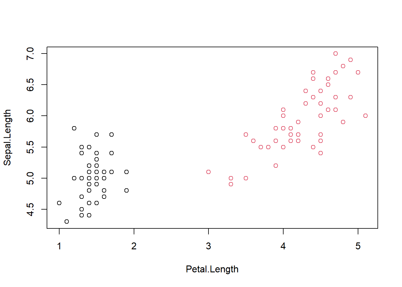
is.setosa = as.factor(ifelse(iris$Species == "setosa", "Sim","Não"))
is.versicolor = as.factor(ifelse(iris$Species == "versicolor", "Sim","Não"))
iris2 = tibble(cbind(iris, is.setosa, is.versicolor))
names(iris2)## [1] "Sepal.Length" "Sepal.Width" "Petal.Length" "Petal.Width"
## [5] "Species" "is.setosa" "is.versicolor"modelRegLog02 = glm(is.setosa ~ Sepal.Length+ Sepal.Width + Petal.Length+ Petal.Width, data = iris2, family = binomial)
summary(modelRegLog02)##
## Call:
## glm(formula = is.setosa ~ Sepal.Length + Sepal.Width + Petal.Length +
## Petal.Width, family = binomial, data = iris2)
##
## Deviance Residuals:
## Min 1Q Median 3Q Max
## -3.185e-05 -2.100e-08 -2.100e-08 2.100e-08 3.173e-05
##
## Coefficients:
## Estimate Std. Error z value Pr(>|z|)
## (Intercept) -16.946 457457.106 0 1
## Sepal.Length 11.759 130504.043 0 1
## Sepal.Width 7.842 59415.386 0 1
## Petal.Length -20.088 107724.596 0 1
## Petal.Width -21.608 154350.619 0 1
##
## (Dispersion parameter for binomial family taken to be 1)
##
## Null deviance: 1.9095e+02 on 149 degrees of freedom
## Residual deviance: 3.2940e-09 on 145 degrees of freedom
## AIC: 10
##
## Number of Fisher Scoring iterations: 25modelRegLog03 = glm(is.versicolor ~ Sepal.Length+ Sepal.Width + Petal.Length+ Petal.Width, data = iris2, family = binomial)
summary(modelRegLog03)##
## Call:
## glm(formula = is.versicolor ~ Sepal.Length + Sepal.Width + Petal.Length +
## Petal.Width, family = binomial, data = iris2)
##
## Deviance Residuals:
## Min 1Q Median 3Q Max
## -2.1280 -0.7668 -0.3818 0.7866 2.1202
##
## Coefficients:
## Estimate Std. Error z value Pr(>|z|)
## (Intercept) 7.3785 2.4993 2.952 0.003155 **
## Sepal.Length -0.2454 0.6496 -0.378 0.705634
## Sepal.Width -2.7966 0.7835 -3.569 0.000358 ***
## Petal.Length 1.3136 0.6838 1.921 0.054713 .
## Petal.Width -2.7783 1.1731 -2.368 0.017868 *
## ---
## Signif. codes: 0 '***' 0.001 '**' 0.01 '*' 0.05 '.' 0.1 ' ' 1
##
## (Dispersion parameter for binomial family taken to be 1)
##
## Null deviance: 190.95 on 149 degrees of freedom
## Residual deviance: 145.07 on 145 degrees of freedom
## AIC: 155.07
##
## Number of Fisher Scoring iterations: 5pred02 = predict.glm(modelRegLog02, type = "response")
pred03 = predict.glm(modelRegLog03, type = "response")
predClass = ifelse(pred02>0.5, "setosa", ifelse(pred03>0.5, "versicolor", "virginica"))
predClass = as.factor(predClass)
confusionMatrix(predClass, iris$Species)## Confusion Matrix and Statistics
##
## Reference
## Prediction setosa versicolor virginica
## setosa 50 0 0
## versicolor 0 25 13
## virginica 0 25 37
##
## Overall Statistics
##
## Accuracy : 0.7467
## 95% CI : (0.6693, 0.8141)
## No Information Rate : 0.3333
## P-Value [Acc > NIR] : < 2.2e-16
##
## Kappa : 0.62
##
## Mcnemar's Test P-Value : NA
##
## Statistics by Class:
##
## Class: setosa Class: versicolor Class: virginica
## Sensitivity 1.0000 0.5000 0.7400
## Specificity 1.0000 0.8700 0.7500
## Pos Pred Value 1.0000 0.6579 0.5968
## Neg Pred Value 1.0000 0.7768 0.8523
## Prevalence 0.3333 0.3333 0.3333
## Detection Rate 0.3333 0.1667 0.2467
## Detection Prevalence 0.3333 0.2533 0.4133
## Balanced Accuracy 1.0000 0.6850 0.7450unique(iris$Species)## [1] setosa versicolor virginica
## Levels: setosa versicolor virginica5.2 NAIVE BAYES
library(e1071)
fit = naiveBayes(Species ~., data = iris)
summary(fit)## Length Class Mode
## apriori 3 table numeric
## tables 4 -none- list
## levels 3 -none- character
## isnumeric 4 -none- logical
## call 4 -none- callpredicted = predict(fit, iris)
confusionMatrix(predicted, iris$Species)## Confusion Matrix and Statistics
##
## Reference
## Prediction setosa versicolor virginica
## setosa 50 0 0
## versicolor 0 47 3
## virginica 0 3 47
##
## Overall Statistics
##
## Accuracy : 0.96
## 95% CI : (0.915, 0.9852)
## No Information Rate : 0.3333
## P-Value [Acc > NIR] : < 2.2e-16
##
## Kappa : 0.94
##
## Mcnemar's Test P-Value : NA
##
## Statistics by Class:
##
## Class: setosa Class: versicolor Class: virginica
## Sensitivity 1.0000 0.9400 0.9400
## Specificity 1.0000 0.9700 0.9700
## Pos Pred Value 1.0000 0.9400 0.9400
## Neg Pred Value 1.0000 0.9700 0.9700
## Prevalence 0.3333 0.3333 0.3333
## Detection Rate 0.3333 0.3133 0.3133
## Detection Prevalence 0.3333 0.3333 0.3333
## Balanced Accuracy 1.0000 0.9550 0.95505.3 Arvores de decisão
library(rpart)
library(rpart.plot)
fit <- rpart(Species ~ ., data = iris, method="class")
summary(fit)## Call:
## rpart(formula = Species ~ ., data = iris, method = "class")
## n= 150
##
## CP nsplit rel error xerror xstd
## 1 0.50 0 1.00 1.18 0.05017303
## 2 0.44 1 0.50 0.70 0.06110101
## 3 0.01 2 0.06 0.09 0.02908608
##
## Variable importance
## Petal.Width Petal.Length Sepal.Length Sepal.Width
## 34 31 21 14
##
## Node number 1: 150 observations, complexity param=0.5
## predicted class=setosa expected loss=0.6666667 P(node) =1
## class counts: 50 50 50
## probabilities: 0.333 0.333 0.333
## left son=2 (50 obs) right son=3 (100 obs)
## Primary splits:
## Petal.Length < 2.45 to the left, improve=50.00000, (0 missing)
## Petal.Width < 0.8 to the left, improve=50.00000, (0 missing)
## Sepal.Length < 5.45 to the left, improve=34.16405, (0 missing)
## Sepal.Width < 3.35 to the right, improve=19.03851, (0 missing)
## Surrogate splits:
## Petal.Width < 0.8 to the left, agree=1.000, adj=1.00, (0 split)
## Sepal.Length < 5.45 to the left, agree=0.920, adj=0.76, (0 split)
## Sepal.Width < 3.35 to the right, agree=0.833, adj=0.50, (0 split)
##
## Node number 2: 50 observations
## predicted class=setosa expected loss=0 P(node) =0.3333333
## class counts: 50 0 0
## probabilities: 1.000 0.000 0.000
##
## Node number 3: 100 observations, complexity param=0.44
## predicted class=versicolor expected loss=0.5 P(node) =0.6666667
## class counts: 0 50 50
## probabilities: 0.000 0.500 0.500
## left son=6 (54 obs) right son=7 (46 obs)
## Primary splits:
## Petal.Width < 1.75 to the left, improve=38.969400, (0 missing)
## Petal.Length < 4.75 to the left, improve=37.353540, (0 missing)
## Sepal.Length < 6.15 to the left, improve=10.686870, (0 missing)
## Sepal.Width < 2.45 to the left, improve= 3.555556, (0 missing)
## Surrogate splits:
## Petal.Length < 4.75 to the left, agree=0.91, adj=0.804, (0 split)
## Sepal.Length < 6.15 to the left, agree=0.73, adj=0.413, (0 split)
## Sepal.Width < 2.95 to the left, agree=0.67, adj=0.283, (0 split)
##
## Node number 6: 54 observations
## predicted class=versicolor expected loss=0.09259259 P(node) =0.36
## class counts: 0 49 5
## probabilities: 0.000 0.907 0.093
##
## Node number 7: 46 observations
## predicted class=virginica expected loss=0.02173913 P(node) =0.3066667
## class counts: 0 1 45
## probabilities: 0.000 0.022 0.978prp(fit,
faclen=0, #use full names for factor labels
extra=1, #display number of observations for each terminal node
roundint=F, #don't round to integers in output
digits=5)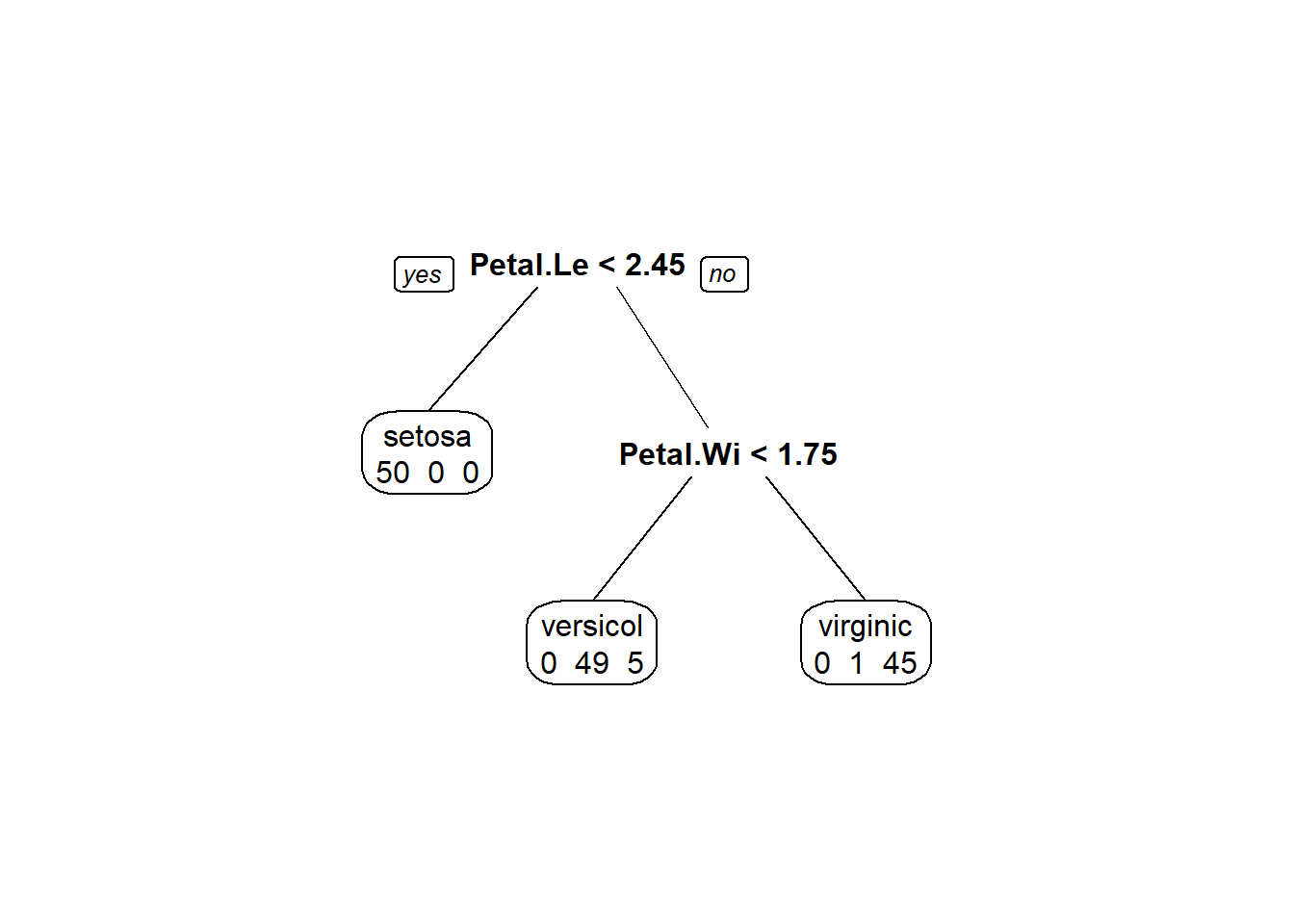
5.3.1 LDA
library(MASS)
iris$Species
## [1] setosa setosa setosa setosa setosa setosa
## [7] setosa setosa setosa setosa setosa setosa
## [13] setosa setosa setosa setosa setosa setosa
## [19] setosa setosa setosa setosa setosa setosa
## [25] setosa setosa setosa setosa setosa setosa
## [31] setosa setosa setosa setosa setosa setosa
## [37] setosa setosa setosa setosa setosa setosa
## [43] setosa setosa setosa setosa setosa setosa
## [49] setosa setosa versicolor versicolor versicolor versicolor
## [55] versicolor versicolor versicolor versicolor versicolor versicolor
## [61] versicolor versicolor versicolor versicolor versicolor versicolor
## [67] versicolor versicolor versicolor versicolor versicolor versicolor
## [73] versicolor versicolor versicolor versicolor versicolor versicolor
## [79] versicolor versicolor versicolor versicolor versicolor versicolor
## [85] versicolor versicolor versicolor versicolor versicolor versicolor
## [91] versicolor versicolor versicolor versicolor versicolor versicolor
## [97] versicolor versicolor versicolor versicolor virginica virginica
## [103] virginica virginica virginica virginica virginica virginica
## [109] virginica virginica virginica virginica virginica virginica
## [115] virginica virginica virginica virginica virginica virginica
## [121] virginica virginica virginica virginica virginica virginica
## [127] virginica virginica virginica virginica virginica virginica
## [133] virginica virginica virginica virginica virginica virginica
## [139] virginica virginica virginica virginica virginica virginica
## [145] virginica virginica virginica virginica virginica virginica
## Levels: setosa versicolor virginicamodBayes01 = lda(Species ~ ., data = iris, prior = c(1/6, 3/6, 2/6))
predito = predict(modBayes01)
confusionMatrix(predito$class, iris$Species)## Confusion Matrix and Statistics
##
## Reference
## Prediction setosa versicolor virginica
## setosa 50 0 0
## versicolor 0 48 1
## virginica 0 2 49
##
## Overall Statistics
##
## Accuracy : 0.98
## 95% CI : (0.9427, 0.9959)
## No Information Rate : 0.3333
## P-Value [Acc > NIR] : < 2.2e-16
##
## Kappa : 0.97
##
## Mcnemar's Test P-Value : NA
##
## Statistics by Class:
##
## Class: setosa Class: versicolor Class: virginica
## Sensitivity 1.0000 0.9600 0.9800
## Specificity 1.0000 0.9900 0.9800
## Pos Pred Value 1.0000 0.9796 0.9608
## Neg Pred Value 1.0000 0.9802 0.9899
## Prevalence 0.3333 0.3333 0.3333
## Detection Rate 0.3333 0.3200 0.3267
## Detection Prevalence 0.3333 0.3267 0.3400
## Balanced Accuracy 1.0000 0.9750 0.9800modFisher01 = lda(Species ~ ., data = iris, prior = c(1/3, 1/3, 1/3))
predito = predict(modFisher01)
confusionMatrix(predito$class, iris$Species)## Confusion Matrix and Statistics
##
## Reference
## Prediction setosa versicolor virginica
## setosa 50 0 0
## versicolor 0 48 1
## virginica 0 2 49
##
## Overall Statistics
##
## Accuracy : 0.98
## 95% CI : (0.9427, 0.9959)
## No Information Rate : 0.3333
## P-Value [Acc > NIR] : < 2.2e-16
##
## Kappa : 0.97
##
## Mcnemar's Test P-Value : NA
##
## Statistics by Class:
##
## Class: setosa Class: versicolor Class: virginica
## Sensitivity 1.0000 0.9600 0.9800
## Specificity 1.0000 0.9900 0.9800
## Pos Pred Value 1.0000 0.9796 0.9608
## Neg Pred Value 1.0000 0.9802 0.9899
## Prevalence 0.3333 0.3333 0.3333
## Detection Rate 0.3333 0.3200 0.3267
## Detection Prevalence 0.3333 0.3267 0.3400
## Balanced Accuracy 1.0000 0.9750 0.98005.3.2 KNN
ModKnn01 = knn3(Species ~ ., data = iris, k = 2)
pred = predict(ModKnn01, iris, type = "class")
confusionMatrix(pred, iris$Species)
## Confusion Matrix and Statistics
##
## Reference
## Prediction setosa versicolor virginica
## setosa 50 0 0
## versicolor 0 48 2
## virginica 0 2 48
##
## Overall Statistics
##
## Accuracy : 0.9733
## 95% CI : (0.9331, 0.9927)
## No Information Rate : 0.3333
## P-Value [Acc > NIR] : < 2.2e-16
##
## Kappa : 0.96
##
## Mcnemar's Test P-Value : NA
##
## Statistics by Class:
##
## Class: setosa Class: versicolor Class: virginica
## Sensitivity 1.0000 0.9600 0.9600
## Specificity 1.0000 0.9800 0.9800
## Pos Pred Value 1.0000 0.9600 0.9600
## Neg Pred Value 1.0000 0.9800 0.9800
## Prevalence 0.3333 0.3333 0.3333
## Detection Rate 0.3333 0.3200 0.3200
## Detection Prevalence 0.3333 0.3333 0.3333
## Balanced Accuracy 1.0000 0.9700 0.9700ModKnn02 = knn3(Species ~ ., data = iris, k = 3)
pred = predict(ModKnn01, iris, type = "class")
confusionMatrix(pred, iris$Species)## Confusion Matrix and Statistics
##
## Reference
## Prediction setosa versicolor virginica
## setosa 50 0 0
## versicolor 0 48 2
## virginica 0 2 48
##
## Overall Statistics
##
## Accuracy : 0.9733
## 95% CI : (0.9331, 0.9927)
## No Information Rate : 0.3333
## P-Value [Acc > NIR] : < 2.2e-16
##
## Kappa : 0.96
##
## Mcnemar's Test P-Value : NA
##
## Statistics by Class:
##
## Class: setosa Class: versicolor Class: virginica
## Sensitivity 1.0000 0.9600 0.9600
## Specificity 1.0000 0.9800 0.9800
## Pos Pred Value 1.0000 0.9600 0.9600
## Neg Pred Value 1.0000 0.9800 0.9800
## Prevalence 0.3333 0.3333 0.3333
## Detection Rate 0.3333 0.3200 0.3200
## Detection Prevalence 0.3333 0.3333 0.3333
## Balanced Accuracy 1.0000 0.9700 0.9700ModKnn03 = knn3(Species ~ ., data = iris, k = 5)
pred = predict(ModKnn01, iris, type = "class")
confusionMatrix(pred, iris$Species)## Confusion Matrix and Statistics
##
## Reference
## Prediction setosa versicolor virginica
## setosa 50 0 0
## versicolor 0 48 1
## virginica 0 2 49
##
## Overall Statistics
##
## Accuracy : 0.98
## 95% CI : (0.9427, 0.9959)
## No Information Rate : 0.3333
## P-Value [Acc > NIR] : < 2.2e-16
##
## Kappa : 0.97
##
## Mcnemar's Test P-Value : NA
##
## Statistics by Class:
##
## Class: setosa Class: versicolor Class: virginica
## Sensitivity 1.0000 0.9600 0.9800
## Specificity 1.0000 0.9900 0.9800
## Pos Pred Value 1.0000 0.9796 0.9608
## Neg Pred Value 1.0000 0.9802 0.9899
## Prevalence 0.3333 0.3333 0.3333
## Detection Rate 0.3333 0.3200 0.3267
## Detection Prevalence 0.3333 0.3267 0.3400
## Balanced Accuracy 1.0000 0.9750 0.9800#SVM
library(e1071)
fit <-svm(Species ~ ., data = iris)
summary(fit)
##
## Call:
## svm(formula = Species ~ ., data = iris)
##
##
## Parameters:
## SVM-Type: C-classification
## SVM-Kernel: radial
## cost: 1
##
## Number of Support Vectors: 51
##
## ( 8 22 21 )
##
##
## Number of Classes: 3
##
## Levels:
## setosa versicolor virginica# plot(fit$SV)
#Predict Output
predicted= predict(fit)
cm = confusionMatrix(as.factor(predicted), iris$Species)
print(cm)## Confusion Matrix and Statistics
##
## Reference
## Prediction setosa versicolor virginica
## setosa 50 0 0
## versicolor 0 48 2
## virginica 0 2 48
##
## Overall Statistics
##
## Accuracy : 0.9733
## 95% CI : (0.9331, 0.9927)
## No Information Rate : 0.3333
## P-Value [Acc > NIR] : < 2.2e-16
##
## Kappa : 0.96
##
## Mcnemar's Test P-Value : NA
##
## Statistics by Class:
##
## Class: setosa Class: versicolor Class: virginica
## Sensitivity 1.0000 0.9600 0.9600
## Specificity 1.0000 0.9800 0.9800
## Pos Pred Value 1.0000 0.9600 0.9600
## Neg Pred Value 1.0000 0.9800 0.9800
## Prevalence 0.3333 0.3333 0.3333
## Detection Rate 0.3333 0.3200 0.3200
## Detection Prevalence 0.3333 0.3333 0.3333
## Balanced Accuracy 1.0000 0.9700 0.9700plot(iris, fit, fill_plot = T, plot_contour = F, plot_decision = T)
n = 300
x1 = runif(n, -5, 5)
x2 = runif(n, -5, 5)
y = factor(ifelse( x1^2+x2^2 <= 9, "Yes", "No"))
data = data.frame(x1,x2,y)

indexes = sample(1:n, size = 0.80*n)
train = data[indexes, ]
test = data[-indexes, ]

xtest = test[, -5]
ytest = test[, 3]

plot(x1~x2, col = y, pch = 16)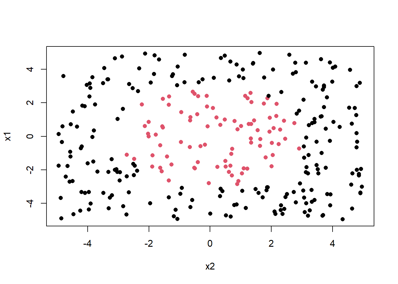
fit <-svm(y ~ ., data = train, kernel = "radial")
summary(fit)
##
## Call:
## svm(formula = y ~ ., data = train, kernel = "radial")
##
##
## Parameters:
## SVM-Type: C-classification
## SVM-Kernel: radial
## cost: 1
##
## Number of Support Vectors: 63
##
## ( 33 30 )
##
##
## Number of Classes: 2
##
## Levels:
## No Yes plot(fit$SV)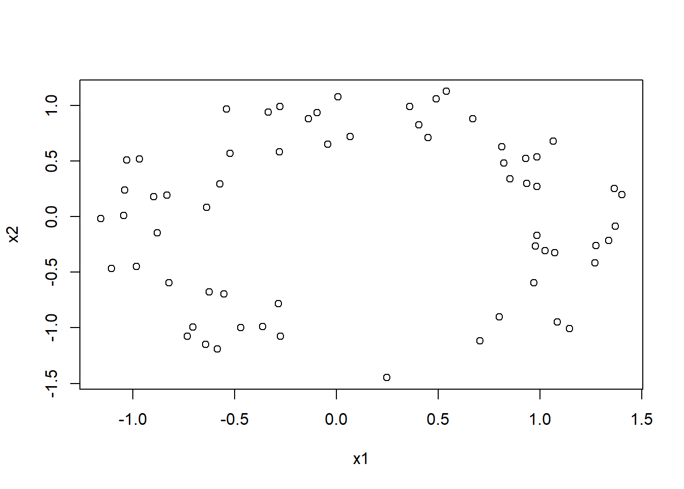
#Predict Output
predicted= predict(fit, test)
cm = confusionMatrix(as.factor(predicted), test$y)
print(cm)
## Confusion Matrix and Statistics
##
## Reference
## Prediction No Yes
## No 46 0
## Yes 0 14
##
## Accuracy : 1
## 95% CI : (0.9404, 1)
## No Information Rate : 0.7667
## P-Value [Acc > NIR] : 1.192e-07
##
## Kappa : 1
##
## Mcnemar's Test P-Value : NA
##
## Sensitivity : 1.0000
## Specificity : 1.0000
## Pos Pred Value : 1.0000
## Neg Pred Value : 1.0000
## Prevalence : 0.7667
## Detection Rate : 0.7667
## Detection Prevalence : 0.7667
## Balanced Accuracy : 1.0000
##
## 'Positive' Class : No
## #Lori::plot_svm_jk(data, fit, fill_plot = T, plot_contour = F, plot_decision = T)5.4 REDES NEURAIS
nnet = neuralnet(Species~., iris, hidden = c(4), linear.output = FALSE)
plot(nnet)

ypred = neuralnet::compute(nnet, iris)
yhat = ypred$net.result


round(yhat)
## [,1] [,2] [,3]
## [1,] 1 0 0
## [2,] 1 0 0
## [3,] 1 0 0
## [4,] 1 0 0
## [5,] 1 0 0
## [6,] 1 0 0
## [7,] 1 0 0
## [8,] 1 0 0
## [9,] 1 0 0
## [10,] 1 0 0
## [11,] 1 0 0
## [12,] 1 0 0
## [13,] 1 0 0
## [14,] 1 0 0
## [15,] 1 0 0
## [16,] 1 0 0
## [17,] 1 0 0
## [18,] 1 0 0
## [19,] 1 0 0
## [20,] 1 0 0
## [21,] 1 0 0
## [22,] 1 0 0
## [23,] 1 0 0
## [24,] 1 0 0
## [25,] 1 0 0
## [26,] 1 0 0
## [27,] 1 0 0
## [28,] 1 0 0
## [29,] 1 0 0
## [30,] 1 0 0
## [31,] 1 0 0
## [32,] 1 0 0
## [33,] 1 0 0
## [34,] 1 0 0
## [35,] 1 0 0
## [36,] 1 0 0
## [37,] 1 0 0
## [38,] 1 0 0
## [39,] 1 0 0
## [40,] 1 0 0
## [41,] 1 0 0
## [42,] 1 0 0
## [43,] 1 0 0
## [44,] 1 0 0
## [45,] 1 0 0
## [46,] 1 0 0
## [47,] 1 0 0
## [48,] 1 0 0
## [49,] 1 0 0
## [50,] 1 0 0
## [51,] 0 1 0
## [52,] 0 1 0
## [53,] 0 1 0
## [54,] 0 1 0
## [55,] 0 1 0
## [56,] 0 1 0
## [57,] 0 1 0
## [58,] 0 1 0
## [59,] 0 1 0
## [60,] 0 1 0
## [61,] 0 1 0
## [62,] 0 1 0
## [63,] 0 1 0
## [64,] 0 1 0
## [65,] 0 1 0
## [66,] 0 1 0
## [67,] 0 1 0
## [68,] 0 1 0
## [69,] 0 1 0
## [70,] 0 1 0
## [71,] 0 1 0
## [72,] 0 1 0
## [73,] 0 1 0
## [74,] 0 1 0
## [75,] 0 1 0
## [76,] 0 1 0
## [77,] 0 1 0
## [78,] 0 1 0
## [79,] 0 1 0
## [80,] 0 1 0
## [81,] 0 1 0
## [82,] 0 1 0
## [83,] 0 1 0
## [84,] 0 0 1
## [85,] 0 1 0
## [86,] 0 1 0
## [87,] 0 1 0
## [88,] 0 1 0
## [89,] 0 1 0
## [90,] 0 1 0
## [91,] 0 1 0
## [92,] 0 1 0
## [93,] 0 1 0
## [94,] 0 1 0
## [95,] 0 1 0
## [96,] 0 1 0
## [97,] 0 1 0
## [98,] 0 1 0
## [99,] 0 1 0
## [100,] 0 1 0
## [101,] 0 0 1
## [102,] 0 0 1
## [103,] 0 0 1
## [104,] 0 0 1
## [105,] 0 0 1
## [106,] 0 0 1
## [107,] 0 0 1
## [108,] 0 0 1
## [109,] 0 0 1
## [110,] 0 0 1
## [111,] 0 0 1
## [112,] 0 0 1
## [113,] 0 0 1
## [114,] 0 0 1
## [115,] 0 0 1
## [116,] 0 0 1
## [117,] 0 0 1
## [118,] 0 0 1
## [119,] 0 0 1
## [120,] 0 0 1
## [121,] 0 0 1
## [122,] 0 0 1
## [123,] 0 0 1
## [124,] 0 0 1
## [125,] 0 0 1
## [126,] 0 0 1
## [127,] 0 0 1
## [128,] 0 0 1
## [129,] 0 0 1
## [130,] 0 0 1
## [131,] 0 0 1
## [132,] 0 0 1
## [133,] 0 0 1
## [134,] 0 0 1
## [135,] 0 0 1
## [136,] 0 0 1
## [137,] 0 0 1
## [138,] 0 0 1
## [139,] 0 0 1
## [140,] 0 0 1
## [141,] 0 0 1
## [142,] 0 0 1
## [143,] 0 0 1
## [144,] 0 0 1
## [145,] 0 0 1
## [146,] 0 0 1
## [147,] 0 0 1
## [148,] 0 0 1
## [149,] 0 0 1
## [150,] 0 0 1yhat=data.frame("yhat"=ifelse(max.col(yhat[ ,1:3])==1, "setosa",
ifelse(max.col(yhat[ ,1:3])==2, "versicolor", "virginica")))
cm = confusionMatrix(as.factor(iris$Species), as.factor(yhat$yhat))
print(cm)## Confusion Matrix and Statistics
##
## Reference
## Prediction setosa versicolor virginica
## setosa 50 0 0
## versicolor 0 49 1
## virginica 0 0 50
##
## Overall Statistics
##
## Accuracy : 0.9933
## 95% CI : (0.9634, 0.9998)
## No Information Rate : 0.34
## P-Value [Acc > NIR] : < 2.2e-16
##
## Kappa : 0.99
##
## Mcnemar's Test P-Value : NA
##
## Statistics by Class:
##
## Class: setosa Class: versicolor Class: virginica
## Sensitivity 1.0000 1.0000 0.9804
## Specificity 1.0000 0.9901 1.0000
## Pos Pred Value 1.0000 0.9800 1.0000
## Neg Pred Value 1.0000 1.0000 0.9900
## Prevalence 0.3333 0.3267 0.3400
## Detection Rate 0.3333 0.3267 0.3333
## Detection Prevalence 0.3333 0.3333 0.3333
## Balanced Accuracy 1.0000 0.9950 0.9902