Chapter 3 Analise das Ações (Graficos e Descritivo)
Carregar pacotes e bibliotecas
#install.packages("bookdown")
#library(bookdown)

if(!require(pacman)) install.packages("pacman")
library(pacman)

pacman::p_load(stringr, ipred, recipes, tidyverse, caret, MASS, readxl, ggthemes, plotly,  rstatix, lmtest, ggpubr, dplyr, ggplot2, corrplot, lubridate, tibble, e1071, neuralnet, remotes, rmarkdown )
Setar pasta
getwd()## [1] "C:/Mestrado/Cadernos_Julio"#
setwd("C:/Mestrado/Cadernos_Julio")3.1 Laboratorio 1
3.1.1 BLOCO 1: R básico
- Calcule as seguintes expressoes no R:
- 12 + (16-7)x7-8/4
Resul = 12 + (16-7) * 7 - 9 / 4- Multiplique a sua idade por meses e salve o resultado em um objeto chamado idade_em_meses.
idade_em_meses = 51 * 12
print(idade_em_meses)
## [1] 6122.1 - Em seguida, multiplique esse objeto por 30 e salve o resultado em um objeto chamado idade_em_dias.
idade_em_dias = idade_em_meses * 30- Guarde em um objeto chamado nome uma string contendo o seu nome completo
nome = "Julio Cesar Vieira"

nome = "Julio"
SobreNome = "Vieira"
NomeCompleto <- str_c(nome," ",SobreNome)- Qual é a soma dos números de 101 a 1000?
sum( 101:1000 )## [1] 495450- Quantos algarismos possui o resultado do produto dos números de 1 a 12?
  #Cria um objeto dianamico de n=12
  for(coluna in 1:12)
  {
    x[[coluna]] <- c( coluna )
  }
  #lista Elementos do Vetor
  print(x)
## [1] 1.0 2.0 3.0 4.0 5.0 6.0 7.0 8.0 9.0 10.0 11.0 12.0 1.2 1.3 1.4
## [16] 1.5 1.6 1.7 1.8 1.9 2.0 2.1 2.2 2.3 2.4 2.5 2.6 2.7 2.8 2.9
## [31] 3.0 3.1 3.2 3.3 3.4 3.5 3.6 3.7 3.8 3.9 4.0 4.1 4.2 4.3 4.4
## [46] 4.5 4.6 4.7 4.8 4.9 5.0 5.1 5.2 5.3 5.4 5.5 5.6 5.7 5.8 5.9
## [61] 6.0 6.1 6.2 6.3 6.4 6.5 6.6 6.7 6.8 6.9 7.0 7.1 7.2 7.3 7.4
## [76] 7.5 7.6 7.7 7.8 7.9 8.0 8.1 8.2 8.3 8.4 8.5 8.6 8.7 8.8 8.9
## [91] 9.0 9.1 9.2 9.3 9.4 9.5 9.6 9.7 9.8 9.9 10.0 10.1 10.2 10.3 10.4
## [106] 10.5 10.6 10.7 10.8 10.9 11.0 11.1 11.2 11.3 11.4 11.5 11.6 11.7 11.8 11.9
## [121] 12.0 12.1 12.2 12.3 12.4 12.5 12.6 12.7 12.8 12.9 13.0 13.1 13.2 13.3 13.4
## [136] 13.5 13.6 13.7 13.8 13.9 14.0 14.1 14.2 14.3 14.4 14.5 14.6 14.7 14.8 14.9
## [151] 15.0 15.1 15.2 15.3 15.4 15.5 15.6 15.7 15.8 15.9 16.0 16.1 16.2 16.3 16.4
## [166] 16.5 16.6 16.7 16.8 16.9 17.0 17.1 17.2 17.3 17.4 17.5 17.6 17.7 17.8 17.9
## [181] 18.0 18.1 18.2 18.3 18.4 18.5 18.6 18.7 18.8 18.9 19.0 19.1 19.2 19.3 19.4
## [196] 19.5 19.6 19.7 19.8 19.9 20.0 20.1 20.2 20.3 20.4 20.5 20.6 20.7 20.8 20.9
## [211] 21.0 21.1 21.2 21.3 21.4 21.5 21.6 21.7 21.8 21.9 22.0 22.1 22.2 22.3 22.4
## [226] 22.5 22.6 22.7 22.8 22.9 23.0 23.1 23.2 23.3 23.4 23.5 23.6 23.7 23.8 23.9
## [241] 24.0 24.1 24.2 24.3 24.4 24.5 24.6 24.7 24.8 24.9 25.0 25.1 25.2 25.3 25.4
## [256] 25.5 25.6 25.7 25.8 25.9 26.0 26.1 26.2 26.3 26.4 26.5 26.6 26.7 26.8 26.9
## [271] 27.0 27.1 27.2 27.3 27.4 27.5 27.6 27.7 27.8 27.9 28.0 28.1 28.2 28.3 28.4
## [286] 28.5 28.6 28.7 28.8 28.9 29.0 29.1 29.2 29.3 29.4 29.5 29.6 29.7 29.8 29.9
## [301] 30.0 30.1 30.2 30.3 30.4 30.5 30.6 30.7 30.8 30.9 31.0 31.1 31.2 31.3 31.4
## [316] 31.5 31.6 31.7 31.8 31.9 32.0 32.1 32.2 32.3 32.4 32.5 32.6 32.7 32.8 32.9
## [331] 33.0 33.1 33.2 33.3 33.4 33.5 33.6 33.7 33.8 33.9 34.0 34.1 34.2 34.3 34.4
## [346] 34.5 34.6 34.7 34.8 34.9 35.0 35.1 35.2 35.3 35.4 35.5 35.6 35.7 35.8 35.9
## [361] 36.0 36.1 36.2 36.3 36.4 36.5 36.6 36.7 36.8 36.9 37.0 37.1 37.2 37.3 37.4
## [376] 37.5 37.6 37.7 37.8 37.9 38.0 38.1 38.2 38.3 38.4 38.5 38.6 38.7 38.8 38.9
## [391] 39.0 39.1 39.2 39.3 39.4 39.5 39.6 39.7 39.8 39.9 40.0 #retorna o produto do Vetor
prod(x)## [1] Inf- Use o vetor números abaixo para responder as questões seguintes:
numeros <- -4:26.1 - Escreva um código que devolva apenas valores positivos do vetor numeros.
numeros[numeros > 0]## [1] 1 26.2. - Escreva um código que de volta apenas os valores pares do vetor numeros.
numeros[numeros %% 2 == 0]## [1] -4 -2 0 26.3 - Filtre o vetor para que retorne apenas aqueles valores que, quando elevados a 2, são menores do que 4.
numeros[numeros^2 < 4]## [1] -1 0 1- Quais as diferenças entre NaN, NULL, NA e Inf? Digite expressões que retornem cada um desses valores.
NaN
numeros <- c( 0, NaN , "F", NaN , 3 )
sum(is.nan(numeros))
## [1] 0Null
numeros <- c( NULL, 3 )
sum(is.null(numeros))
## [1] 0NA
numeros <- c( NA, 2 )
sum(is.na(numeros))
## [1] 1- Carregue o conjunto de dados airquality com o comando data(airquality) para responder às questões abaixo.
3.2 Laboratorio 2
3.2.1 BLOCO 1: R básico
Carregar o conjunto de dados inibina
getwd()## [1] "C:/Mestrado/Cadernos_Julio"inibina <- read_excel("Dados/inibina.xls")
nrow(inibina)## [1] 32sum()## [1] 0inibina$difinib = inibina$inibpos - inibina$inibpre
#agrupar as respostas e contador a qtde
inibina$resposta = as.factor(inibina$resposta)
plot(inibina$difinib ~ inibina$resposta, ylim = c(0,400))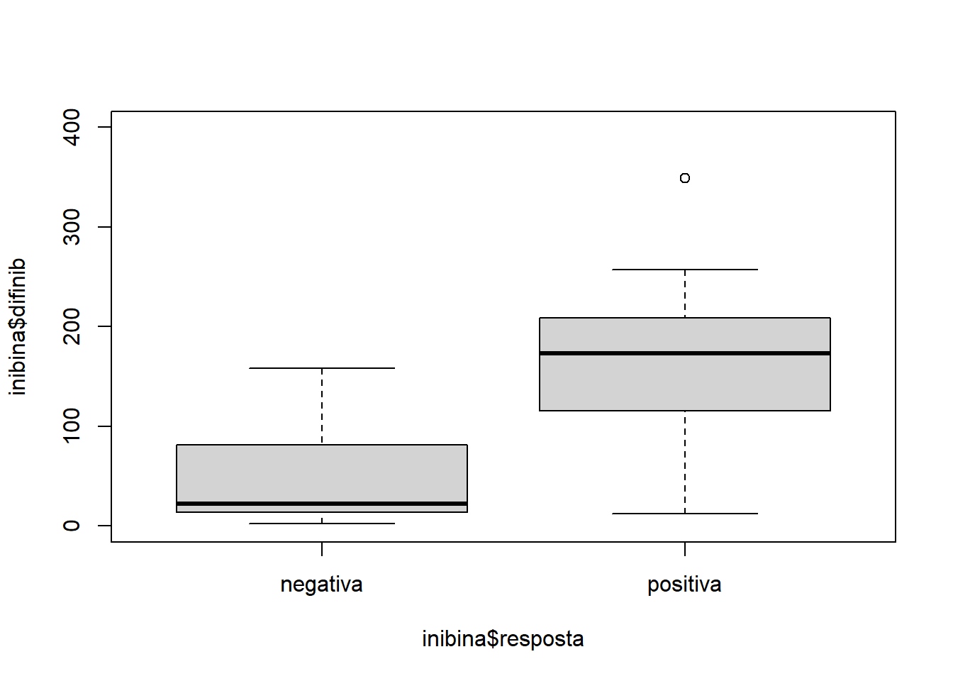
# Hmisc::describe(inibina)

summary(inibina)
## ident resposta inibpre inibpos
## Min. : 1.00 negativa:13 Min. : 3.02 Min. : 6.03
## 1st Qu.: 8.75 positiva:19 1st Qu.: 52.40 1st Qu.: 120.97
## Median :16.50 Median :109.44 Median : 228.89
## Mean :16.50 Mean :100.53 Mean : 240.80
## 3rd Qu.:24.25 3rd Qu.:148.93 3rd Qu.: 330.77
## Max. :32.00 Max. :186.38 Max. :1055.19
## difinib
## Min. : 2.48
## 1st Qu.: 24.22
## Median :121.18
## Mean :140.27
## 3rd Qu.:183.77
## Max. :868.81sd( inibina$difinib )## [1] 159.2217modLogist01 = glm( resposta ~ difinib, family = binomial, data = inibina )
summary( modLogist01 )##
## Call:
## glm(formula = resposta ~ difinib, family = binomial, data = inibina)
##
## Deviance Residuals:
## Min 1Q Median 3Q Max
## -1.9770 -0.5594 0.1890 0.5589 2.0631
##
## Coefficients:
## Estimate Std. Error z value Pr(>|z|)
## (Intercept) -2.310455 0.947438 -2.439 0.01474 *
## difinib 0.025965 0.008561 3.033 0.00242 **
## ---
## Signif. codes: 0 '***' 0.001 '**' 0.01 '*' 0.05 '.' 0.1 ' ' 1
##
## (Dispersion parameter for binomial family taken to be 1)
##
## Null deviance: 43.230 on 31 degrees of freedom
## Residual deviance: 24.758 on 30 degrees of freedom
## AIC: 28.758
##
## Number of Fisher Scoring iterations: 6#c. Ajuste um modelo de regressão logística aos dados. Qual é a acurácia do modelo em fazer classificação?
predito = predict.glm( modLogist01, type = "response")
classPred = ifelse(predito>0.5,"positiva", "negativa")
classPred = as.factor(classPred)
confusionMatrix(classPred, inibina$resposta, positive = "positiva" )## Confusion Matrix and Statistics
##
## Reference
## Prediction negativa positiva
## negativa 10 2
## positiva 3 17
##
## Accuracy : 0.8438
## 95% CI : (0.6721, 0.9472)
## No Information Rate : 0.5938
## P-Value [Acc > NIR] : 0.002273
##
## Kappa : 0.6721
##
## Mcnemar's Test P-Value : 1.000000
##
## Sensitivity : 0.8947
## Specificity : 0.7692
## Pos Pred Value : 0.8500
## Neg Pred Value : 0.8333
## Prevalence : 0.5938
## Detection Rate : 0.5312
## Detection Prevalence : 0.6250
## Balanced Accuracy : 0.8320
##
## 'Positive' Class : positiva
## #d.Use o classificador linear de Fisher para classificar a variável resposta de acordo com a variável preditora. Qual é a acurácia do classificador?
modFisher01 = lda( resposta ~ difinib, data = inibina, prior = c(0.5 , 0.5))
predito = predict(modFisher01)
confusionMatrix(classPred, inibina$resposta, positive = "positiva")## Confusion Matrix and Statistics
##
## Reference
## Prediction negativa positiva
## negativa 10 2
## positiva 3 17
##
## Accuracy : 0.8438
## 95% CI : (0.6721, 0.9472)
## No Information Rate : 0.5938
## P-Value [Acc > NIR] : 0.002273
##
## Kappa : 0.6721
##
## Mcnemar's Test P-Value : 1.000000
##
## Sensitivity : 0.8947
## Specificity : 0.7692
## Pos Pred Value : 0.8500
## Neg Pred Value : 0.8333
## Prevalence : 0.5938
## Detection Rate : 0.5312
## Detection Prevalence : 0.6250
## Balanced Accuracy : 0.8320
##
## 'Positive' Class : positiva
## #e. Use o classificador linear de Bayes para classificar a variável resposta de acordo com as variáveis explicativas. Utilize priori 0,65 e 0,35 para resposta negativa e positiva, respectivamente. Qual é a acurácia do classificador?
#Use o classificador knn para classificar a variável resposta de acordo com as variáveis preditoras. Utilize k = 1, 3, 5.
#library(iris)
#iris = tibble(iris)
#iris$ = iris[,1:4]3.3 Laboratorio - Aula 3
Carga Excel
dadoscenario1 = read_excel("Dados/Data_HousePrice_Area.xlsx", sheet = 1)
dadoscenario2 = read_excel("Dados/Data_HousePrice_Area.xlsx", sheet = 2)
  ## Lendo e arrumando o conjunto de dados
series = read_excel("Dados/03 B1 ESTATISTICAS DESC E REGRESSAO.xlsx", sheet = 2, n_max = 1)
nomes = names(series)[seq(1,20,2)]
series = read_excel("Dados/03 B1 ESTATISTICAS DESC E REGRESSAO.xlsx", sheet = 2, skip = 1)
names(series)[seq(1,20,2)] = paste0("DATA_", nomes)
names(series)[seq(2,20,2)] = nomes
series
## # A tibble: 3,147 × 20
## DATA_ELET3 ELET3 DATA_ITUB4 ITUB4 DATA_ITSA4 ITSA4
## <dttm> <dbl> <dttm> <dbl> <dttm> <dbl>
## 1 2010-01-04 16:56:00 37.4 2010-01-04 16:56:00 20.1 2010-01-04 16:56:00 8.05
## 2 2010-01-05 16:56:00 37.1 2010-01-05 16:56:00 20.2 2010-01-05 16:56:00 8.02
## 3 2010-01-06 16:56:00 36.6 2010-01-06 16:56:00 20.0 2010-01-06 16:56:00 7.92
## 4 2010-01-07 16:56:00 37.4 2010-01-07 16:56:00 19.8 2010-01-07 16:56:00 7.88
## 5 2010-01-08 16:56:00 38.1 2010-01-08 16:56:00 19.5 2010-01-08 16:56:00 7.82
## 6 2010-01-11 16:56:00 37.5 2010-01-11 16:56:00 19.4 2010-01-11 16:56:00 7.79
## 7 2010-01-12 16:56:00 37.1 2010-01-12 16:56:00 19.2 2010-01-12 16:56:00 7.79
## 8 2010-01-13 16:56:00 37.5 2010-01-13 16:56:00 19.2 2010-01-13 16:56:00 7.77
## 9 2010-01-14 16:56:00 36.9 2010-01-14 16:56:00 19.0 2010-01-14 16:56:00 7.66
## 10 2010-01-15 16:56:00 35.6 2010-01-15 16:56:00 18.7 2010-01-15 16:56:00 7.47
## # … with 3,137 more rows, and 14 more variables: DATA_PETR4 <dttm>,
## # PETR4 <dbl>, DATA_NUBR33 <dttm>, NUBR33 <dbl>, DATA_MGLU3 <dttm>,
## # MGLU3 <dbl>, DATA_BBDC4 <dttm>, BBDC4 <dbl>, DATA_VALE3 <dttm>,
## # VALE3 <dbl>, DATA_BBAS3 <dttm>, BBAS3 <dbl>, DATA_LREN3 <dttm>, LREN3 <dbl>Selecionando um subconjunto do conjunto de dados
for (i in seq(1,20,2)) {
    series[[i]] = as.Date(series[[i]])
}
3.3.1 Performance de algumas ações
plot(x=series$DATA_ELET3, y= series$ELET3, type = "l", xlab = "Tempo (dias)", ylab = "Preço fechamento (R$)", main = "Performance de algumas ações ao longo do tempo", ylim = c(0, 60) )
lines(x=series$DATA_ITUB4, y= series$ITUB4, col = 2)
lines(x=series$DATA_PETR4, y= series$PETR4, col = 3)
lines(x=series$DATA_NUBR33, y= series$NUBR33, col = 4)
legend("topleft", legend = c("ELET3", "ITUB4", "PETR4", "NUBR33"), fill = c(1,2,3,4))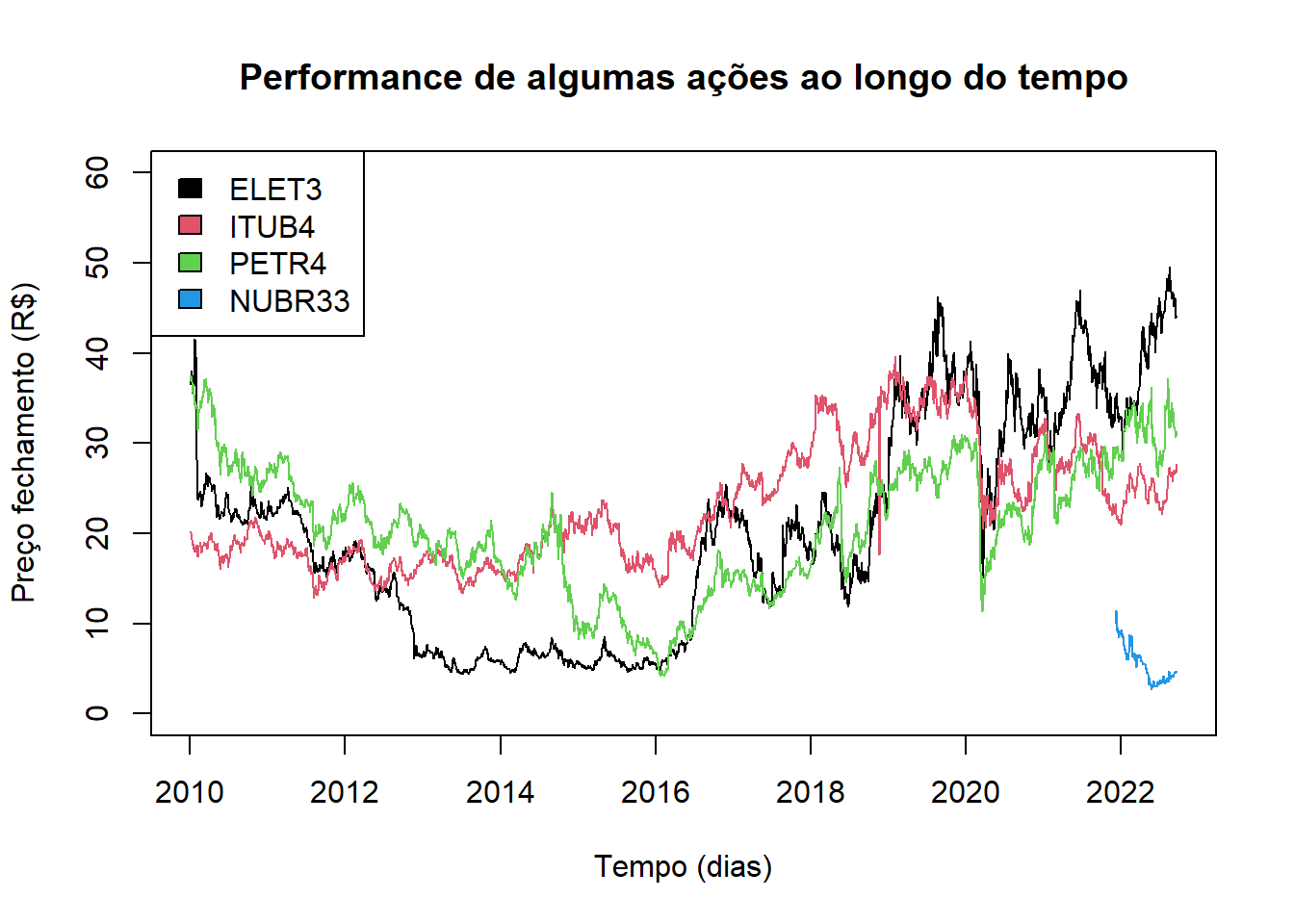 O for seguinte transforma o tipo das colunas de Datetime para apenas Date.
dataInicial = as.Date("2020-01-01")
dataFinal  = as.Date("2021-01-01")
subConjunto = filter(series, DATA_ITUB4 >= dataInicial & DATA_ITUB4 <= dataFinal)
#Fazendo mais gráficos e criandos as estatísticas
Data = subConjunto$DATA_ITUB4
Ser = subConjunto$ITUB4
media = mean(Ser, na.rm = T)
media
## [1] 26.91806desvio = sd(Ser, na.rm = T)
desvio## [1] 4.125498plot(x=Data, y= Ser, type = "l", xlab = "Tempo (dias)", ylab = "Preço fechamento (R$)")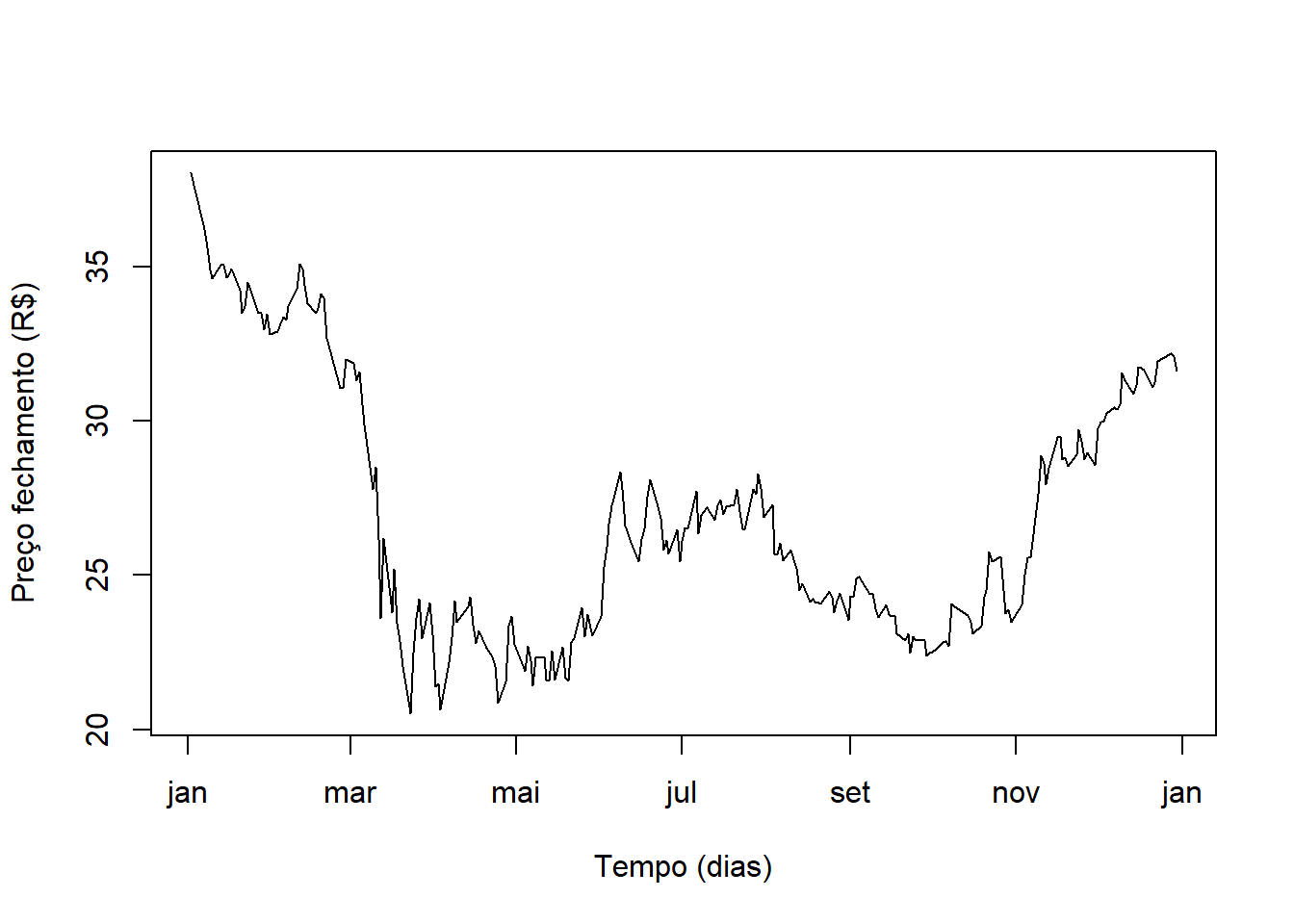
plot(Ser ~ Data, type = "l", xlab = "Tempo (dias)", ylab = "Preço fechamento (R$)", ylim = c(-10, 80))
abline(h = media)
abline(h = media + 1*desvio, col = 2, lwd = 2)
abline(h = media - 1*desvio, col = 2, lwd = 2)
abline(h = media + 2*desvio, col = 3, lwd = 2)
abline(h = media - 2*desvio, col = 3, lwd = 2)

caixa = boxplot(Ser, add = T)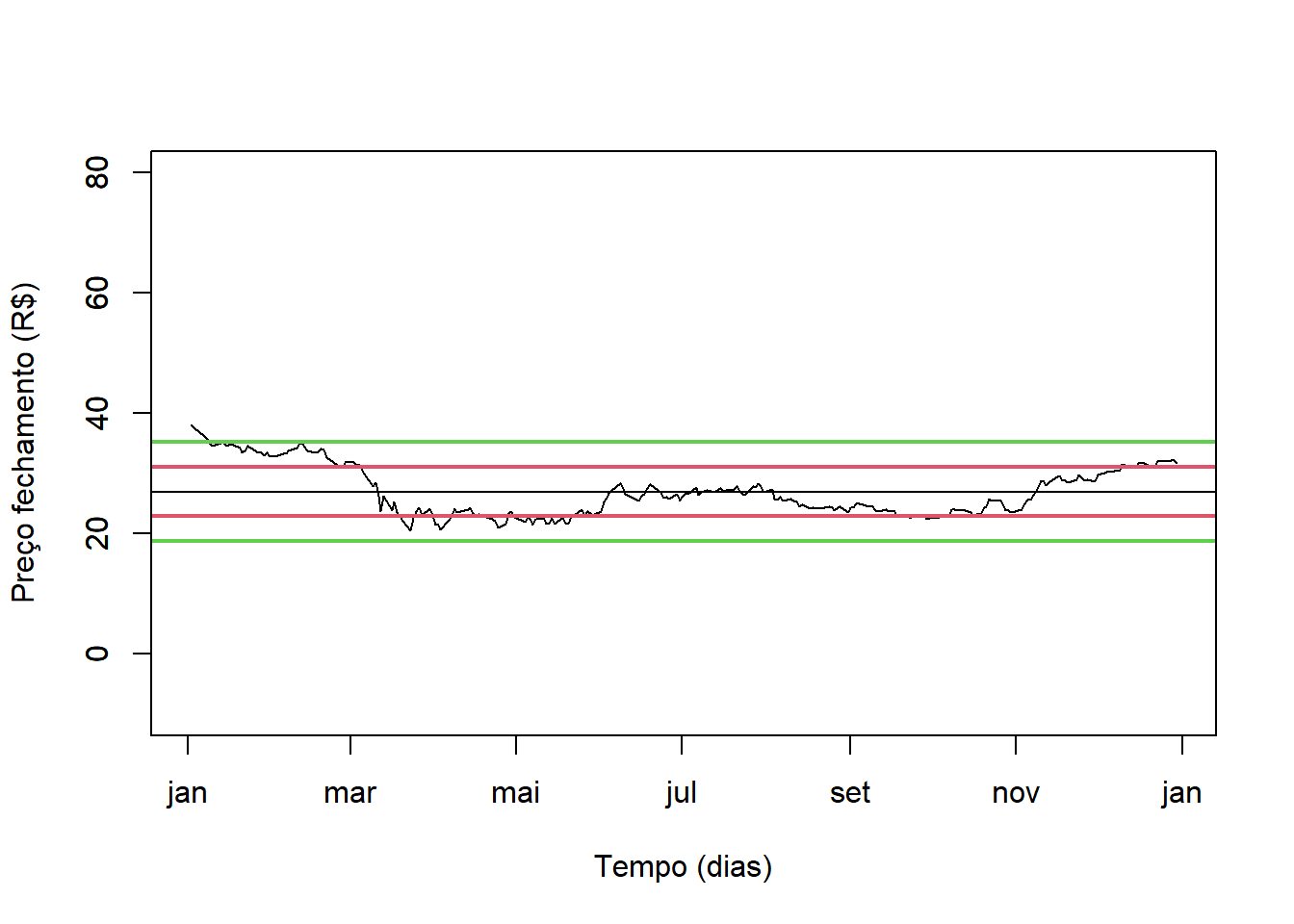
caixa## $stats
## [,1]
## [1,] 20.520
## [2,] 23.615
## [3,] 25.840
## [4,] 29.915
## [5,] 38.030
##
## $n
## [1] 247
##
## $conf
## [,1]
## [1,] 25.20664
## [2,] 26.47336
##
## $out
## numeric(0)
##
## $group
## numeric(0)
##
## $names
## [1] "1"limSup = caixa$stats[5,1]
Q3 = caixa$stats[4,1]
Q2 = caixa$stats[3,1]
Q1 = caixa$stats[2,1]
limInf = caixa$stats[1,1]
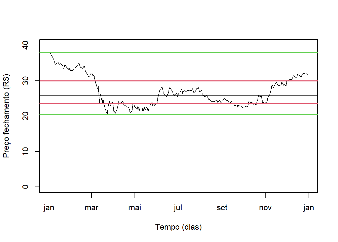
plot(Ser ~ Data, type = "l", xlab = "Tempo (dias)", ylab = "Preço fechamento (R$)", ylim = c(-0, 40))
abline(h = Q2)
abline(h = Q3, col = 2, lwd = 2)
abline(h = Q1, col = 2, lwd = 2)
abline(h = limSup, col = 3, lwd = 2)
abline(h = limInf, col = 3, lwd = 2)