6 Nonparametric Regression
Consider the general Regression Problem \[Y=m(X)+\epsilon\] where \(Y\) (response) and \(X\) (covariate) are real-valued random variables andwe assume to have data \((Y_i,X_i),...,(Y_n,X_n)\) such that \((Y_i,X_i)\sim F_{X,Y}\). Observe that (as long as \(Y\) has finite expectation), this model always holds!
6.1 Polynomial Regression
In linear regression, we make an assumption that \(m\) is linear, that is \[m(x)=\beta_0+\beta_1x\] for some unknown \(\beta_0,\beta_1\in \mathbb R\). If this relation holds, we can find \(\hat \beta_0\) and \(\hat \beta_1\) that minimize the least squared error \[\sum_{i=1}^n(Y_i-\beta_0-\beta_1 X_i)^2\] that is, the OLS estimator. Very often, however, the a priori assumed linear relation is too simple. \begin{example} We want to infer on the effect of fertilizer (\(X\)) on crop yield (\(Y\)). We observe the data (in in Kg/ha)
x<-c(801,913,501,767,98,8,484)## amount of fertilizer
y<-c(68.13 ,  85.26 , 68.01 , 73.30 , 51.14 ,  37.15 , 74.29)# Crop Yield
The OLS estimates for \(\hat \beta_0\) and \(\hat \beta_1\) are (approx)
lm(y~x)$coefficients## (Intercept) x
## 44.07862674 0.04163763One can also plot the corresponding regression line
grid<-seq(0,1000, by = 10)
plot(x=grid, y=(44.08+ 0.04*grid), type = "l", ylab = "Crop Yield", xlab = "Fertilizer")
points(x=x, y=y)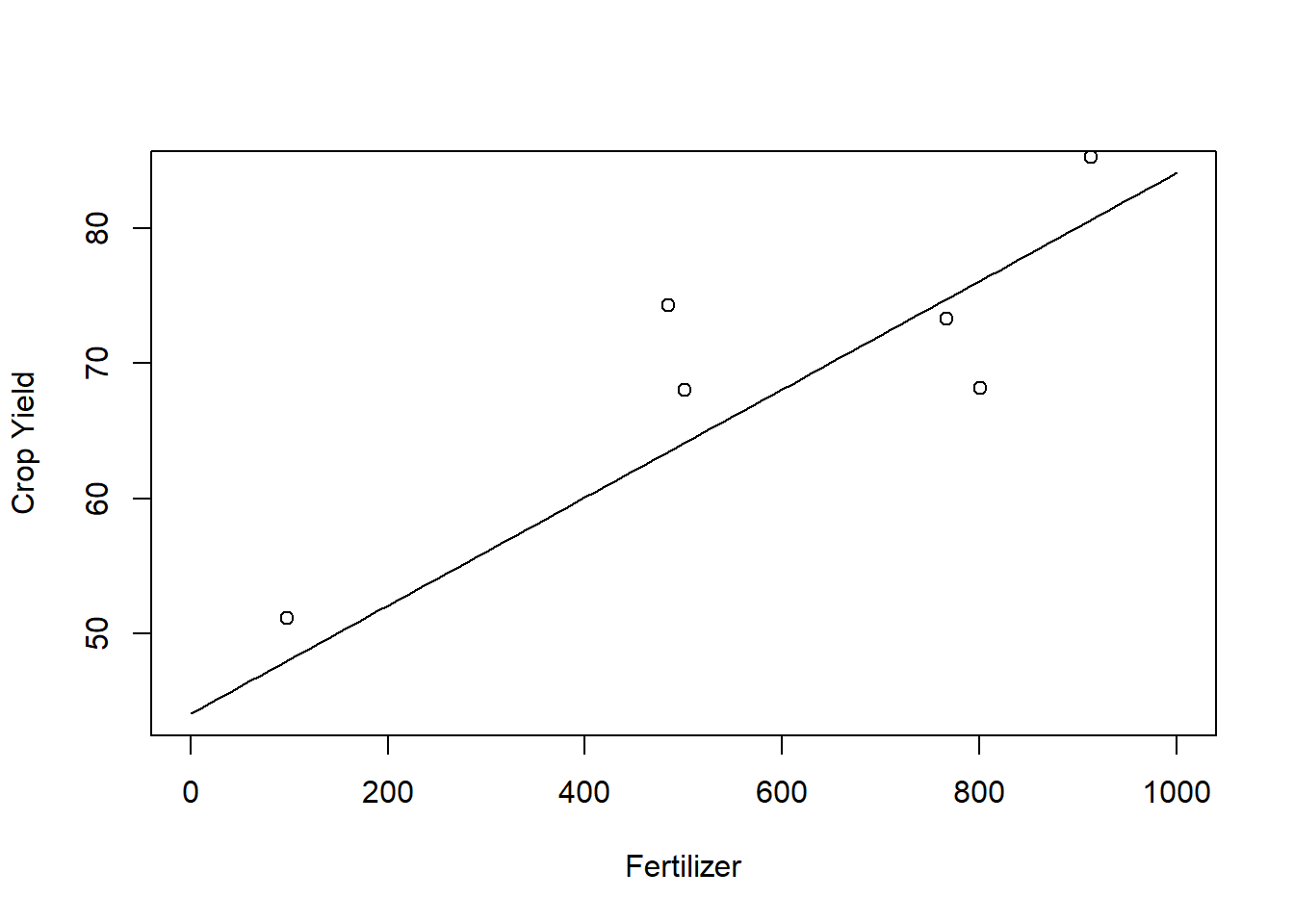
This model predicts that the more fertilizer we use, the better the crop yield will be. However, this is not realistic and at some point we might expect the crop yield to deteriorate. Assume we also observe the additional data:
x.add<-c(x, 1435 , 1165 ,  1255 , 1125 , 1308)## amount of fertilizer
y.add<-c(y,58.12 , 78.29 , 57.44 , 73.38 , 80.44)# Crop Yield
The fitted regression taking into account the new data is plotted below as the solid line and the old one is depicted as the dashed line.
###new linear regression
lm(y.add~x.add)$coefficients
## (Intercept) x.add
## 54.52784570 0.01527544grid.add<-seq(0,1500, by = 10)
plot(x=grid.add, y=(44.08+ 0.04*grid.add), type = "l", ylab = "crop yield", xlab = "amount of fertilizer", lty =2)
lines(x=grid.add, y=(54.53+ 0.015*grid.add), type = "l")
points(x=x.add, y=y.add)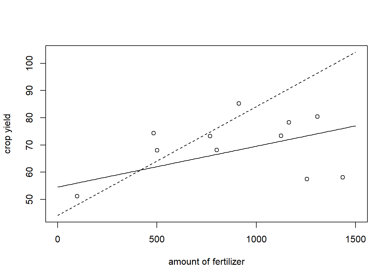
The regression line using only the old data looks quite misspecified, the one that uses all the data looks a bit better. However, especially for low and high values of fertilizer, the prediction is not particularly good as well. The problem is that the data do not really indicate a linear relation between \(Y\) and \(X\).
A possible way out is to still use linear models, but to allow the regression curve to have other shapes than linear. for instance, one might fit a quadratic relation and assume \[m(x)=\beta_0+\beta_1 x+\beta_2 x^2.\] In that case, we can still use the OLS Estimator to derive
lm(y.add~poly(x.add,2,raw=TRUE))$coefficients## (Intercept) poly(x.add, 2, raw = TRUE)1 poly(x.add, 2, raw = TRUE)2
## 39.528880345 0.085859379 -0.000049017Especially at the ends of the curves, the prediction seems to be better than for the regression line:
plot(x=grid.add, y=(39.52+ 0.085*grid.add+-0.00005*grid.add^2),ylim = c(30,90), type = "l", ylab = "crop yield", xlab = "amount of fertilizer")
lines(x=grid.add, y=(54.53+ 0.015*grid.add), type = "l", lty =2)
points(x=x.add, y=y.add)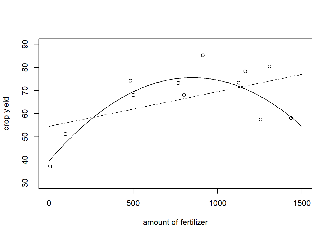
The previous example indicates that increasing the complexity of the model can sometimes help to achieve better predictions. Why don’t we just assume a very high polynomial degree \(p\), such that the model can fit very intricate patterns perfectly?
Assume that we assume the degree of the polynomial is \(p =10\), that is, \[m(x)=\beta_{10}x^{10}+...+\beta_1 x +\beta_0?\] In this case, the model could recognize any polynomial relationship up to order \(10\), but the fit does not look very pleasing.
LM.10<-lm(y.add~poly(x.add,10, raw = TRUE))$coefficients
length(grid.add)
## [1] 151fit<-numeric(151)+as.numeric(LM.10[1])
for (i in 1:10){
fit<-fit + as.numeric(LM.10[i+1])*(grid.add^i)
}
plot(x=grid.add, y=fit, type = "l", ylab = "crop yield", xlab = "amount of fertilizer")
points(x=x.add, y=y.add)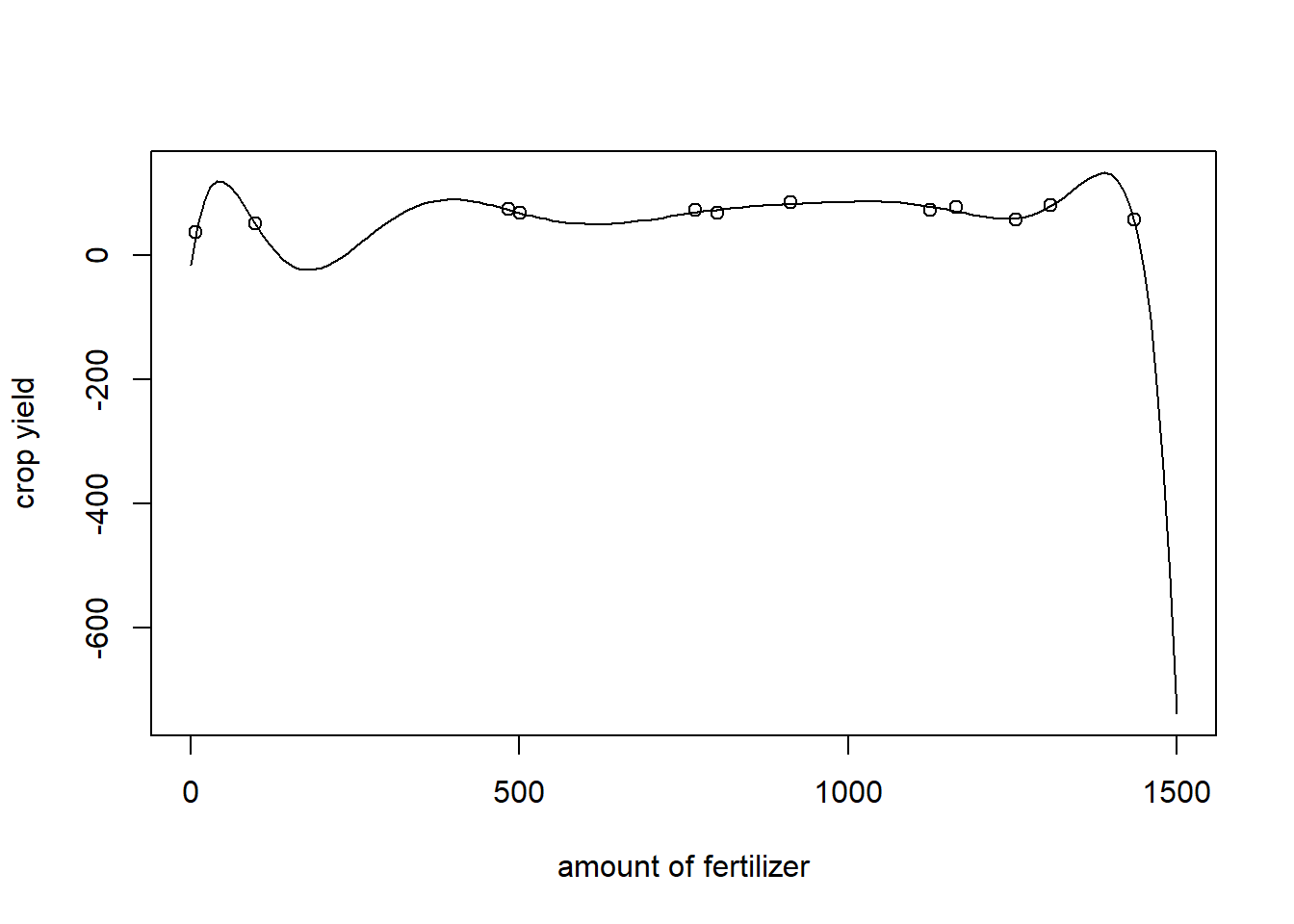
Obviously, the model overfits the data. Indeed, if we would have left just one point out of the regression, the fitted curve would look very different.
LM.10.Lastleftout<-lm(y.add[-12]~poly(x.add[-12],10,raw =TRUE))$coefficients
fit.Lastleftout<-numeric(151)+as.numeric(LM.10.Lastleftout[1])
for (i in 1:10){
fit.Lastleftout<-fit.Lastleftout + as.numeric(LM.10.Lastleftout[i+1])*(grid.add^i)
}
plot(x=grid.add, y=fit.Lastleftout, type = "l", ylab = "crop yield", xlab = "amount of fertilizer")
points(x=x.add, y=y.add)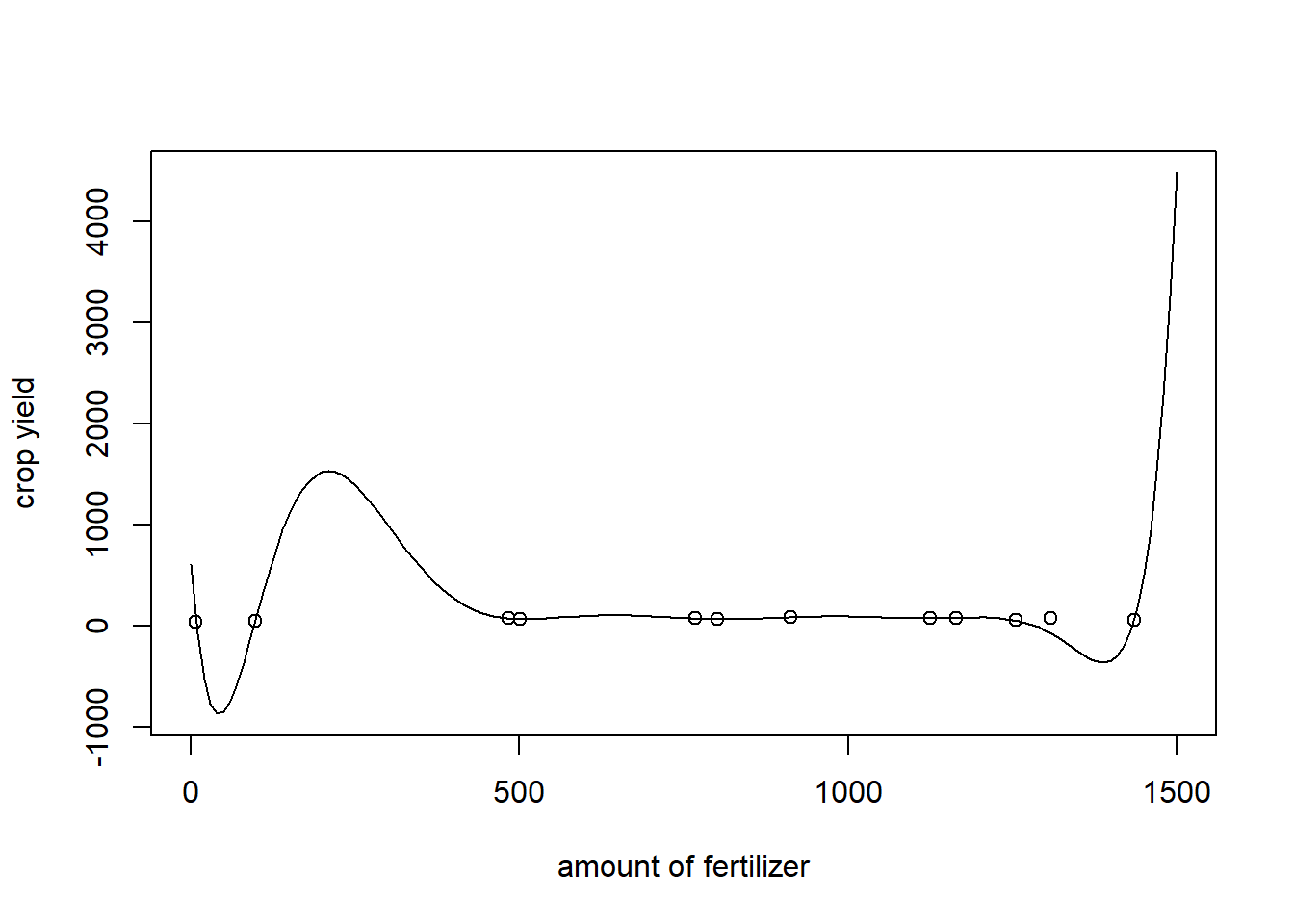 The predicted value for the point that was left out is approximately \(-70.55\), while the corresponding value is \(80.44\). Arguably, using a polynomial of degree 10 would lead to very unreliable predictions.
How can we decide on the bases of the data, which model we should choose? This is quite difficult in general one thing we could do is derive an adequate degree of the polynomial ba cross-validation. that is, we choose \(p\in \mathbb N\) such that it minimizes \[CV(p)=\sum_{i=1}^n(Y_i-m_{p,-i}(X_i))^2\] where \(m_{p,-i}\) is the fitted (via OLS) regression polynomial of order \(p\) based on the data \((Y_1,X_1),...,(Y_{i-1},X_{i-1}),(Y_{i+1},X_{i+1}),...,(Y_n,X_n)\).
While in practise the cross-validations yields a reasonable criterion to choose the polynomial degree, one can also interpret theoretically why choosing a degree that is unnecessarily high leads to bad results. Ideed, one can show that the MSE of the OLS estimator is \[MASE=\mathbb E\left[\sum_{i=1}^n (m_p(X_i)-\hat m_p(X_i))^2\right]=\frac{(p+1)\sigma^2}n.\]
Often, however, polynomial relations are not an adequate assumption and polynomials are not adequate basis functions for a series estimator. Another way is to use purely nonparametric kernel estimators.
6.2 Nadaraya Watson Estimators
The idea of the local kernel estimators is to estimate values of \(m(x)\) for different \(x\) by a weighted average of sampled response values, weighting points that correspond to an \(X_i\)-value which is close to \(x\) higher than others. Precisely, the Nadaraya-Watson estimator takes the form \[\hat m_h(x)=\frac 1{nh} \sum_{i=1}^n\frac{K\left(\frac{x-X_j}{h}\right)}{\sum_{j=1}^nK \left(\frac{x-X_i}{h}\right)}Y_i,\] where There are many possible choices for kernels, but popular ones includeKernel estimators which use the Gaussian kernel take into account all available data to estimate a point \(m(x)\), while the estimators using the Epanechnikov or the biweight kernel just take into account \(X_i\)’s whose distance to \(x\) is lower than \(h\). While an adequate choice of a kernel is important, it is crucial to choose an appropriate bandwidth \(h\). If the bandwidth is chosen too low, kernel estimators tend to overfit the data, while a bandwidth that is too high oversmoothes.