1 Introduction to R
This tutorial serves two purposes. First, I will introduce the software package R. Second, we will use R to review very basic concepts in statistics and linear algebra that will be important for the theoretical components of the class.
This script relies on two main sources:
- The past script of Prof. Dr. Dominik Liebl
- The online textbook Introduction to Econometrics with R
Other very good and much more exhaustive tutorials and useful reference-cards can be found at the following links:
- Reference card for R commands (always useful)
- Matlab/R reference (for those who are familiar with Matlab)
- The official Introduction to R (very detailed)
- And many more at www.r-project.org (see “Documents”)
- An R-package for learning R: www.swirl.com
- An excellent book project which covers also advanced issues such as “writing performant code” and “package development”: adv-r.had.co.nz
- Another excellent book: R for Data Science
- An introduction to statistical learning with R
- ChatGPT
Some other tutorials:
Why R?
- R is free of charge from: www.r-project.org
- The celebrated IDE RStudio for R is also free of charge: www.rstudio.com
- R is equipped with one of the most flexible and powerful graphics routines available anywhere.
For instance, check out one of the following repositories: - R is a standard for statistical science.
- R has been used in other classes.
1.1 Short Glossary
Make sure that RStudio is installed on your computer before the next lecture. When you work with RStudio, it is typically split in 4 panels as illustrated in the figure below.
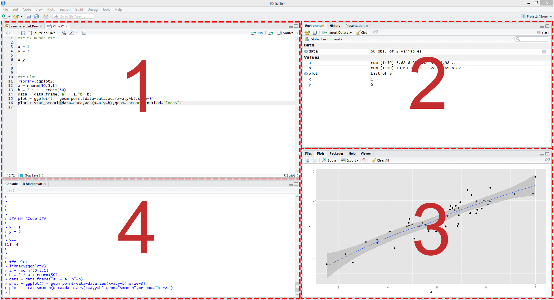
Figure 1: Illustration of RStudio
These panels show:
- Your script file, which is an ordinary text file with suffix “.R”. For instance, yourFavoritFileName.R. This file contains your code.
- All objects we have defined in the environment.
- Help files and plots.
- The console, which allows you to type commands and display results.
Some other terms I will refer to are:
- Working directory: The file-directory you are working in. Useful commands: with
getwd()you get the location of your current working directory andsetwd()allows you to set a new location for it. - Workspace: This is a hidden file (stored in the working directory), where all objects you use (e.g., data, matrices, vectors, variables, functions, etc.) are stored. Useful commands:
ls()shows all elements in our current workspace andrm(list=ls())deletes all elements in our current workspace.
1.2 First Steps
It will be helpful to use a script file such as yourFavoritFileName.R to store your R commands. You can send single lines or marked regions of your R-code to the console by pressing the keys STRG+ENTER.
To begin with baby steps, do some simple computations:
2+2 # and all the others: *,/,-,^2,^3,... ## [1] 4Note: Everything that is written after the #-sign is ignored by R, which is very useful to comment your code.
The second window above, starting with ##, shows the output.
The assignment operator will be your most often used tool. Here an example to create a scalar variable:
x <- 4
x
## [1] 44 -> x # possible but unusual
x## [1] 4Note: The R community loves the <- assignment operator, which is a very unusual syntax. Alternatively, you can use the = operator:
x = 4 And now a more interesting object - a vector:
y <- c(2,7,4,1)
y
## [1] 2 7 4 1As mentioned, the command ls() shows the total content of your current workspace, and the command rm(list=ls()) deletes all elements of your current workspace:
ls()## [1] "A" "all_eps" "b0"
## [4] "b1" "beta_df" "beta_vec"
## [7] "beta_Ztest_TwoSided" "calc_probs_asymp_normal" "calc_probs_consistency"
## [10] "calc_rej_probs" "data_set" "eps"
## [13] "ind" "lm_result" "lm_result_ln"
## [16] "lm_result_rating" "lm_summary" "lm_summary_ln"
## [19] "lm_summary_rating" "mu_0" "mu_0_vec"
## [22] "mus" "myFirst.Array" "myFirst.Dataframe"
## [25] "myFirst.List" "n" "p"
## [28] "probs" "S" "sigma"
## [31] "t_test_stat" "theta" "theta_hat"
## [34] "x" "X" "X_mean"
## [37] "X_sd" "Xmat" "y"
## [40] "z" "Z"rm(list=ls())
ls()## character(0)Note: RStudio’s environment panel also lists all the elements in your current workspace. That is, the command ls() becomes a bit obsolete when working with RStudio.
Let’s do a very quick linear algebra review. We expect that you are familiar with basic linear algebra, but if you think you need a refresher, there is a summary of some of the key concept on the class website. all those concepts There are three different ways to multiply a vector, namely element by element, using the inner product, or using the outer product. Element by element gives you a vector of the same dimension:
y <- c(2,7,4,1)
y*y
## [1] 4 49 16 1The inner product \(y^\top y\) gives you a number:
t(y) %*% y## [,1]
## [1,] 70and the outer product \(y y^\top\) gives you a matrix:
y %*% t(y)## [,1] [,2] [,3] [,4]
## [1,] 4 14 8 2
## [2,] 14 49 28 7
## [3,] 8 28 16 4
## [4,] 2 7 4 1Notice that R actually stores \(z = y^\top y\) as a matrix, which you can check using
z = t(y) %*% y
class(z)
## [1] "matrix" "array"# and compare to y and x
class(y)## [1] "numeric"x <- 4
class(x)## [1] "numeric"You might think that
t(y) * y## [,1] [,2] [,3] [,4]
## [1,] 4 49 16 1is a more sensible notation to calculate the inner product, but that is not what the command calculates. Instead you could simply use
y %*% y## [,1]
## [1,] 70which can be confusing. Using the transpose explicitly might make it easier to spot mistakes.
Either way, be very careful with %*% versus *.
You can also multiply a vector with a scalar:
x*y # each element in the vector, y, is multiplied by the scalar, x.## [1] 8 28 16 4The term-by-term execution as in the above example, y*y, is actually a central strength of R. We can conduct many operations vector-wise:
y^2## [1] 4 49 16 1log(y)## [1] 0.6931472 1.9459101 1.3862944 0.0000000exp(y)## [1] 7.389056 1096.633158 54.598150 2.718282y-mean(y)## [1] -1.5 3.5 0.5 -2.5(y-mean(y))/sd(y) # standardization ## [1] -0.5669467 1.3228757 0.1889822 -0.9449112This is a central characteristic of so called matrix based languages like R (or Matlab). Other programming languages often have to use loops instead:
N <- length(y)
1:N

y.sq <- numeric(N)
y.sq

for(i in 1:N){
  y.sq[i] <- y[i]^2
}
print(y.sq)
The for()-loop is the most common loop. But there is also a while()-loop and a repeat()-loop. However, loops in R can be rather slow, therefore, try to avoid them!
We discussed the function c() that can be used to combine objects. We have also seen functions to calculate means, standard deviations, and simple monotone transformations of vectors. All function calls use the same general notation: a function name is always followed by round parentheses. Sometimes, the parentheses include arguments, such as:
# generate the vector `z`
z <- seq(from = 1, to = 5, by = 1)

z
## [1] 1 2 3 4 5We have also seen that square brackets are used to refer to particular elements of objects.
Useful commands to produce sequences of numbers:
1:10
-10:10
?seq # Help for the seq()-function
seq(from=1, to=100, by=7)
Instead of typing ?sec, you can also highlight the word seq and press F1 in RStudio.
Next, let’s define a square matrix containing the sequence 1:16. Again, if you are uncertain, type
?matrixWe now define:
A <- matrix(data=1:16, nrow=4, ncol=4)
A
## [,1] [,2] [,3] [,4]
## [1,] 1 5 9 13
## [2,] 2 6 10 14
## [3,] 3 7 11 15
## [4,] 4 8 12 16A <- matrix(1:16, 4, 4)Note that a matrix has always two dimensions, but a vector has only one dimension:
dim(A) # Dimension of matrix A?## [1] 4 4dim(y) # dim() does not operate on vectors.## NULLlength(y) # Length of vector y?## [1] 4You can multiply the matrix element by element A
A*A## [,1] [,2] [,3] [,4]
## [1,] 1 25 81 169
## [2,] 4 36 100 196
## [3,] 9 49 121 225
## [4,] 16 64 144 256or calculate \(AA\), \(A^{\top}A\), or \(AA^{\top}\):
A%*%A## [,1] [,2] [,3] [,4]
## [1,] 90 202 314 426
## [2,] 100 228 356 484
## [3,] 110 254 398 542
## [4,] 120 280 440 600t(A)%*%A## [,1] [,2] [,3] [,4]
## [1,] 30 70 110 150
## [2,] 70 174 278 382
## [3,] 110 278 446 614
## [4,] 150 382 614 846A%*%t(A)## [,1] [,2] [,3] [,4]
## [1,] 276 304 332 360
## [2,] 304 336 368 400
## [3,] 332 368 404 440
## [4,] 360 400 440 480Make sure you understand how all these products are calculated. Understanding basic matrix algebra is extremely important for later parts of this course. We will also frequently use matrix-vector-multiplication:
A%*%y## [,1]
## [1,] 86
## [2,] 100
## [3,] 114
## [4,] 128As we have seen in the loop above, the []-operator selects elements of vectors and matrices:
A[,1]
A[4,4]
y[c(1,4)]
This can be done on a more logical basis, too. For example, if you want to know which elements in the first column of matrix A are strictly greater than 2:
# See which elements:
A[,1]>2
## [1] FALSE FALSE TRUE TRUE# and extract the elements
A[A[,1]>2,1]## [1] 3 4Note: Logical operations return so-called boolean objects, i.e., either a TRUE or a FALSE. For instance, if we ask R whether 1>2 we get the answer FALSE.
1.3 Further Data Objects
Besides classical data objects such as scalars, vectors, and matrices there are three further data objects in R:
1. The array: As a matrix but with more dimensions. Here is an example of a \(2\times 2\times 2\)-dimensional array:
myFirst.Array <- array(c(1:8), dim=c(2,2,2)) # Take a look at it!
2. The list: In lists you can organize different kinds of data. E.g., consider the following example:
myFirst.List <- list("Some_Numbers" = c(66, 76, 55, 12, 4, 66, 8, 99),
                     "Animals"      = c("Rabbit", "Cat", "Elefant"),
                     "My_Series"    = c(30:1))
A very useful function to find specific values and entries within lists is the str()-function:
str(myFirst.List)## List of 3
## $ Some_Numbers: num [1:8] 66 76 55 12 4 66 8 99
## $ Animals : chr [1:3] "Rabbit" "Cat" "Elefant"
## $ My_Series : int [1:30] 30 29 28 27 26 25 24 23 22 21 ...
3. The data frame: A data.frame is a list-object but with some more formal restrictions (e.g., equal number of rows for all columns). As indicated by its name, a data.frame-object is designed to store data:
myFirst.Dataframe <- data.frame("Credit_Default"   = c( 0, 0, 1, 0, 1, 1),
                                "Age"              = c(35,41,55,36,44,26),
                                "Loan_in_1000_EUR" = c(55,65,23,12,98,76))
# Take a look at it!
1.4 Simple Statistical Analysis
This section reviews some basic concepts of probability theory and statistics and demonstrates how they can be applied in R.
Most of the statistical functionalities in R are collected in the stats package. It provides simple functions which compute descriptive measures and facilitate computations involving a variety of probability distributions. It also contains more sophisticated routines that, e.g., enable the user to estimate a large number of models based on the same data or help to conduct extensive simulation studies. stats is part of the base distribution of R, meaning that it is installed by default.
As we will see later, more advanced packages have to be installed (here, for example, by running install.packages(“stats”)) and loaded at the beginning of your script (here with library(“stats”)). This is not necessary here, but we will return to this issue later.
Simply execute library(help = “stats”) in the console to view the documentation and a complete list of all functions gathered in stats. For most packages a documentation that can be viewed within RStudio is available. Documentations can be invoked using the ? operator, e.g., upon execution of ?stats the documentation of the stats package is shown in the help tab of the bottom-right panel.
Hopefully, you have learnt about random variables, distribution functions, density functions, and their features, such as means and covariances, before. If you think that you need a refresher, please look at chapter 2 of Introduction to Econometrics with R.
To get started, let \(X\) be a random variable with cumulative distribution function \(F_X\), expected value \(E(X)\), and variance \(Var(X)\). In econometrics, we often deal with random samples of size \(n\), which is a collection of \(n\) independent and identically distributed random variables. We denote a random sample from \(F_X\) by \(\{X_1, X_2, \ldots, X_n\}\).
Taking random samples from common distributions is very simple in R. Let’s start by taking one draw from a uniform distribution on \([0,1]\):
runif(1, min = 0, max = 1) ## [1] 0.0125258or simply
runif(1, 0, 1) ## [1] 0.07452156To make sure that we can replicate the results, it is useful to set a seed:
set.seed(5361)Next, take \(n = 10\) draws and save them in a vector called X:
n <- 10
X <- runif(n, min = 0, max = 1)
We can now calculate the sample average and the sample variance by
mean(X)## [1] 0.5390876var(X)## [1] 0.09811052Here and in the calculations below, it is always useful to think about whether the results are similar to those you would have expected.
You can draw from other distributions using functions such as rnorm or rbinom. For most standard distribution, simply google and you will find the answer immediately.
Returning to the uniform distribution, let’s take \(S = 1000\) random samples, store them in a matrix, check the dimension, and look at the first 5 columns:
S <- 1000
Xmat <- (replicate(S, runif(n,min = 0, max = 1)))
dim(Xmat)
## [1] 10 1000Xmat[,1:5]## [,1] [,2] [,3] [,4] [,5]
## [1,] 0.3772679 0.3936593 0.2256218 0.9816715 0.1103659
## [2,] 0.4799448 0.9957699 0.2586843 0.7364337 0.4934012
## [3,] 0.1494130 0.8753569 0.9573955 0.5968432 0.8202912
## [4,] 0.8867919 0.5019701 0.5295651 0.9949933 0.4850010
## [5,] 0.8106065 0.2503730 0.2819786 0.1128055 0.2669051
## [6,] 0.4806385 0.1550478 0.9950450 0.9119757 0.9534558
## [7,] 0.3004647 0.3333629 0.2471203 0.1047303 0.4140936
## [8,] 0.7351444 0.5166166 0.1920343 0.8958205 0.5021418
## [9,] 0.8530291 0.7747603 0.5942305 0.0629392 0.4378487
## [10,] 0.9581616 0.8784750 0.2263411 0.5624745 0.2121423Next, we will take the sample average for each of the \(S = 1000\) samples, by simply calculating the sample average for each column:
Z <- colMeans(Xmat)The vector \(Z\) now contains \(1000\) sample averages. Let’s look at a histogram:
hist(Z,xlab = "Sample Average", col = "steelblue", xlim = c(0,1))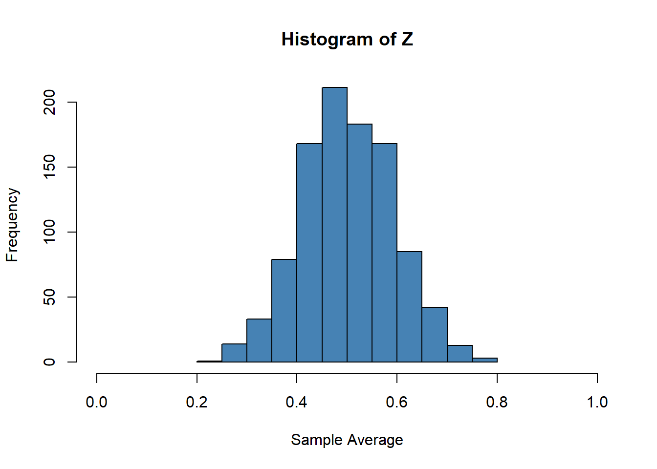
Check the help file to see the different histogram options. The sample average and sample variance of the sample of sample averages are
mean(Z)## [1] 0.501604var(Z)## [1] 0.008503969Again, think about if those results are consistent with the statistical theory you know. Also think about (and try it on your own) how the results will change when \(n= 100\) instead of \(n=10\).
1.5 Regression Analysis
You have all learnt about the linear regression model in your econometrics class where \[Y = \beta_0 + \beta_1 X_1 + \beta_2 X_2 + \ldots + \beta_K X_K + \varepsilon \] and \[E(\varepsilon \mid X_1, X_2, \ldots, X_K) = 0.\] That is, the conditional mean of the outcome variable \(Y\) is a linear function of the regressors \(X_1, X_2, \ldots, X_K\).
When we have a random sample of size \(n\), we can also write \[Y_i = \beta_0 + \beta_1 X_{i1} + \beta_2 X_{i2} + \ldots + \beta_K X_{iK} + \varepsilon_i, \qquad i = 1, 2, \ldots, n.\] Our goal is to estimate the coefficients \(\beta_0, \beta_1, \ldots, \beta_K\) using the data \(\{Y_i, X_{i1},X_{i2},\ldots, X_{iK}\}^n_{i=1}\).
We will now see how to run regressions in R. To do so, we will use some real data, namely a movie database from IMDB that you can download here. You can also find it on the class website. The data set contains among others the budget, the revenue, and the average rating of movies.
Once the data is saved in your working directory, you can load it using
data_set = read.csv("tmdb_5000_movies.csv")which stores the data in a data frame. You can use the View() function to look the data.
Suppose we are interested in studying how the budget of a movie is related to its revenue and we model the relationship as: \[revenue_i = \beta_0 + \beta_1 budget_{i} + \varepsilon_i\] Before we run a regression, let’s look at a scatter plot of the relevant variables:
plot(data_set$budget, data_set$revenue, xlab = "Budget", ylab = "Revenue")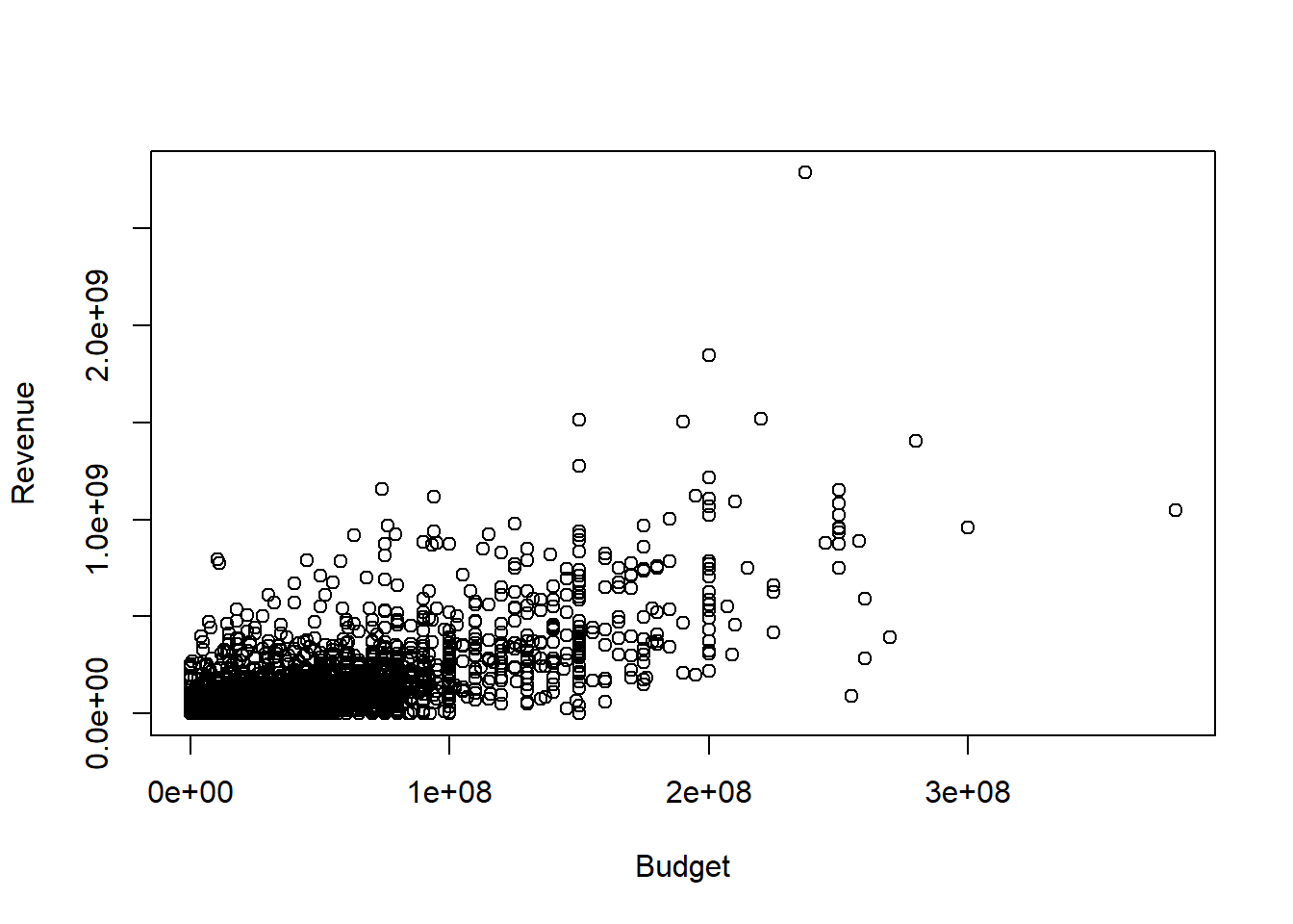
Clearly, movies with higher budgets tend to have higher revenues. To estimate the regression coefficients, you can use the lm() command:
lm_result <- lm(formula = data_set$revenue~data_set$budget)
lm_summary  <- summary(lm_result)
lm_summary
##
## Call:
## lm(formula = data_set$revenue ~ data_set$budget)
##
## Residuals:
## Min 1Q Median 3Q Max
## -653371282 -35365659 2250851 8486969 2097912654
##
## Coefficients:
## Estimate Std. Error t value Pr(>|t|)
## (Intercept) -2.630e+06 1.970e+06 -1.335 0.182
## data_set$budget 2.923e+00 3.940e-02 74.188 <2e-16 ***
## ---
## Signif. codes: 0 '***' 0.001 '**' 0.01 '*' 0.05 '.' 0.1 ' ' 1
##
## Residual standard error: 111200000 on 4801 degrees of freedom
## Multiple R-squared: 0.5341, Adjusted R-squared: 0.534
## F-statistic: 5504 on 1 and 4801 DF, p-value: < 2.2e-16Think about how you can interpret the estimated slope coefficient.
We can also plot the regression line in the scatter plot:
b0 <- lm_summary$coefficients[1]
b1  <- lm_summary$coefficients[2]

## Plot all:
plot(y=data_set$revenue, x=data_set$budget,
     xlab="Budget",
     ylab="Revenue",
     main="Scatter plot and regression line")
abline(a=b0, b=b1, col="red")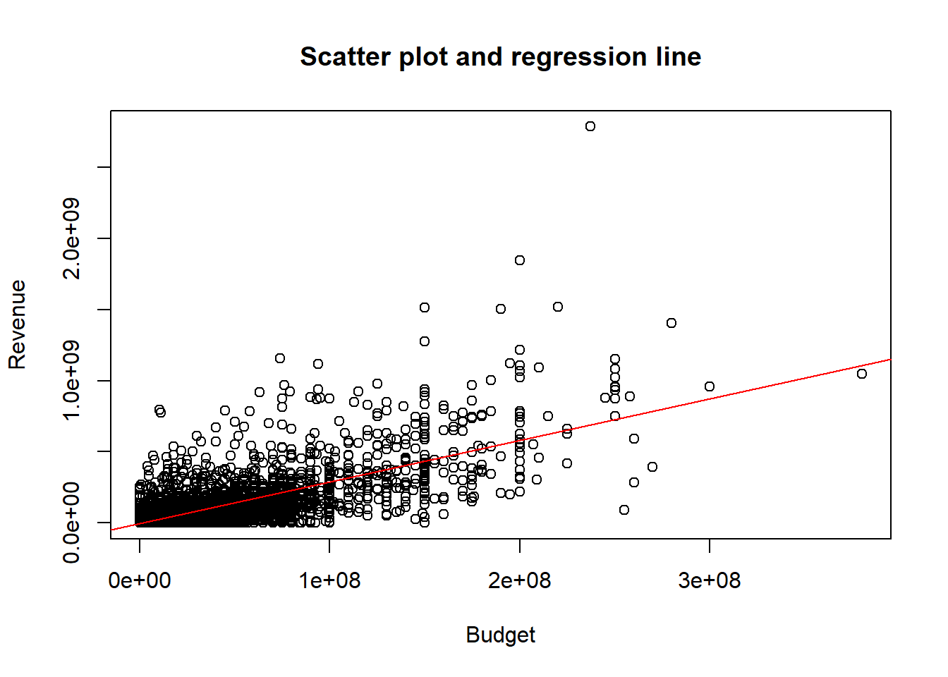
An alternative specification uses logarithms \[\ln(revenue_i) = \beta_0 + \beta_1 \ln(budget_{i}) + \varepsilon_i\] Here we need to focus on movies with strictly positive revenues and budgets. To do so, take
ind = (data_set$budget>0)&(data_set$revenue>0)and run the regression with the relevant subsample:
lm_result_ln <- lm(log(data_set$revenue[ind])~log(data_set$budget[ind]))
lm_summary_ln <- summary(lm_result_ln)
lm_summary_ln
##
## Call:
## lm(formula = log(data_set$revenue[ind]) ~ log(data_set$budget[ind]))
##
## Residuals:
## Min 1Q Median 3Q Max
## -15.1303 -0.6376 0.2259 0.8481 12.2493
##
## Coefficients:
## Estimate Std. Error t value Pr(>|t|)
## (Intercept) 3.70628 0.27975 13.25 <2e-16 ***
## log(data_set$budget[ind]) 0.82054 0.01657 49.52 <2e-16 ***
## ---
## Signif. codes: 0 '***' 0.001 '**' 0.01 '*' 0.05 '.' 0.1 ' ' 1
##
## Residual standard error: 1.569 on 3227 degrees of freedom
## Multiple R-squared: 0.4318, Adjusted R-squared: 0.4316
## F-statistic: 2452 on 1 and 3227 DF, p-value: < 2.2e-16Again, think about how you can interpret the estimated slope coefficient.
Let’s also plot the results:
## Plot all:
plot(y=log(data_set$revenue[ind]), x=log(data_set$budget[ind]),
     xlab="Logarithm of Budget",
     ylab="Logarithm of Revenue",
     main="Scatter plot and regression line")
abline(a=lm_summary_ln$coefficients[1], b=lm_summary_ln$coefficients[2], col="red")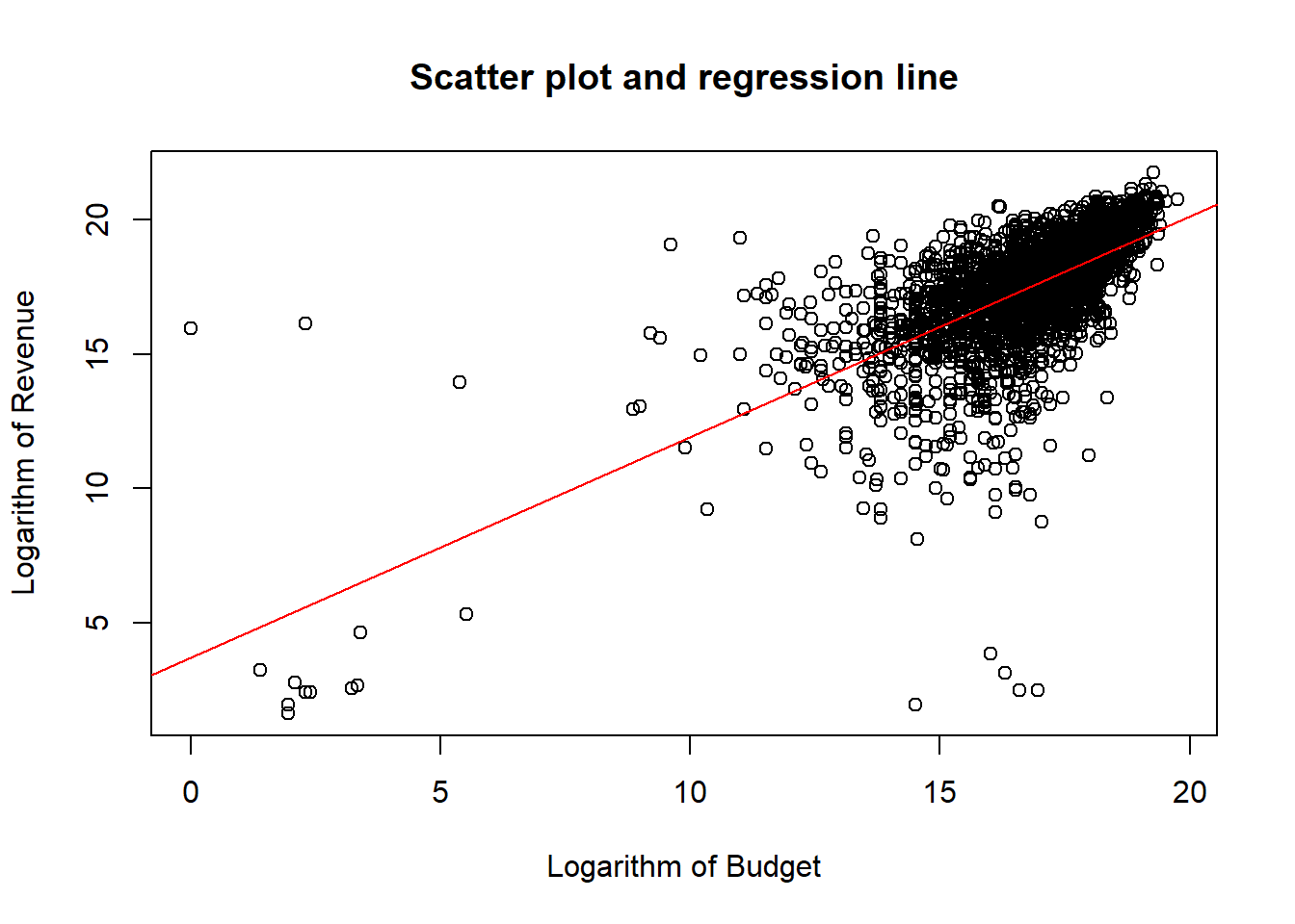
Finally, let’s see if a higher budget also implies a higher rating:
lm_result_rating <- lm(data_set$vote_average~data_set$budget)
lm_summary_rating  <- summary(lm_result_rating)
lm_summary_rating
##
## Call:
## lm(formula = data_set$vote_average ~ data_set$budget)
##
## Residuals:
## Min 1Q Median 3Q Max
## -6.0224 -0.5131 0.1139 0.7462 3.9872
##
## Coefficients:
## Estimate Std. Error t value Pr(>|t|)
## (Intercept) 6.013e+00 2.108e-02 285.190 < 2e-16 ***
## data_set$budget 2.732e-09 4.215e-10 6.482 9.95e-11 ***
## ---
## Signif. codes: 0 '***' 0.001 '**' 0.01 '*' 0.05 '.' 0.1 ' ' 1
##
## Residual standard error: 1.19 on 4801 degrees of freedom
## Multiple R-squared: 0.008676, Adjusted R-squared: 0.00847
## F-statistic: 42.02 on 1 and 4801 DF, p-value: 9.949e-11Notice that the estimated slope coefficient is tiny. Does that mean that the rating is unrelated to the budget?
The budget is often huge. For a better interpretation of the coefficients, define the budget in millions as
data_set$budget_mil <- data_set$budget/1000000look at summary statistics of the variables
summary(data_set$vote_average)## Min. 1st Qu. Median Mean 3rd Qu. Max.
## 0.000 5.600 6.200 6.092 6.800 10.000summary(data_set$budget_mil )## Min. 1st Qu. Median Mean 3rd Qu. Max.
## 0.00 0.79 15.00 29.05 40.00 380.00and redo the analysis:
lm_result_rating <- lm(formula = data_set$vote_average~data_set$budget_mil)
lm_summary_rating  <- summary(lm_result_rating)
lm_summary_rating
##
## Call:
## lm(formula = data_set$vote_average ~ data_set$budget_mil)
##
## Residuals:
## Min 1Q Median 3Q Max
## -6.0224 -0.5131 0.1139 0.7462 3.9872
##
## Coefficients:
## Estimate Std. Error t value Pr(>|t|)
## (Intercept) 6.0128066 0.0210835 285.190 < 2e-16 ***
## data_set$budget_mil 0.0027325 0.0004215 6.482 9.95e-11 ***
## ---
## Signif. codes: 0 '***' 0.001 '**' 0.01 '*' 0.05 '.' 0.1 ' ' 1
##
## Residual standard error: 1.19 on 4801 degrees of freedom
## Multiple R-squared: 0.008676, Adjusted R-squared: 0.00847
## F-statistic: 42.02 on 1 and 4801 DF, p-value: 9.949e-11Do think that the budget has a large impact on the rating?
Of course, we are not limited to one regressors. To include three regressors, can use lm(formula = Y~X1+X2+X3). We will return to regression analysis later in the semester.