3 Statistical Hypothesis Testing

3.1 Hypotheses and Test-Statistics

Let $X_{1}, \ldots, X_{n}$ be a random sample and assume that the distribution of $X_{i}$, depends on some unknown parameter $\theta \in \Theta$, and where $\Theta$ is the parameter space.

General Testing Problem: $$H_{0}: \theta \in \Theta_{0}$$ against $$H_{1}: \theta \in \Theta_{1}$$ $H_{0}$ is the null hypothesis, while $H_{1}$ is the alternative. $\Theta_{0} \subset \Theta$ and $\Theta_{1} \subset \Theta$ are used to denote the possible values of $\theta$ under $H_{0}$ and $H_{1}$. We assume that $\Theta_{0} \cap \Theta_{1}=\emptyset$.

In many cases, the null hypothesis states that $\theta$ is equal to a specific value $\theta_{0} \in \mathbb{R}$, i.e., $\Theta_{0}=\left\{\theta_{0}\right\}$ and the null hypothesis is $H_{0}: \theta=\theta_{0}$. Depending on the alternative one then often distinguishes between one-sided $\left(\Theta_{1}=\left(\theta_{0}, \infty\right)\right.$ or $\left.\Theta_{1}=\left(-\infty, \theta_{0}\right)\right)$ and two-sided tests $\left(\Theta_{1}=\left\{\theta \in \mathbb{R} \mid \theta \neq \theta_{0}\right\}\right)$. The data $X_{1}, \ldots, X_{n}$ is used in order to decide whether or not to reject $H_{0}$.

Test Statistic: Every statistical hypothesis test relies on a corresponding test statistic $$T=T\left(X_{1}, \ldots, X_{n}\right) .$$ Any test statistic is a random variable since it is a deterministic function of random variables. Given realizations $x_{1}, \ldots, x_{n}$ we obtain a realization of the test statistic denote by $$T_{obs}=T\left(x_{1}, \ldots, x_{n}\right) .$$ How can we use $T_{obs}$ to decide between $H_{0}$ and $H_{1}$? Generally, the distribution of $T$ under $H_{0}$ is analyzed in order to define a rejection region $\mathcal C$

For one-sided tests in the scalar case, the rejection rejection $\mathcal C$ is typically of the form either $\left(-\infty, c_{0}\right]$ or $\left[c_{1}, \infty\right)$. For two-sided tests $\mathcal C$ typically takes the form of $\left(-\infty, c_{0}\right] \cup\left[c_{1}, \infty\right)$. The limits $c_{0}$ and $c_{1}$ of the respective intervals are called “critical values”, and are obtained from quantiles of the null distribution, i.e., the distribution of $T$ under $H_{0}$.

3.2 Significance Level, Size and p-Values

We can make two decision errors: (1) Reject a null hypothesis although it is true or (2) fail to reject when null hypothesis is not true

We cannot avoid both errors. Given that we impose an upper bound for the Type I error, we try to minimize the type II error.

Significance Level: In a statistical significance test, the probability of a type I error is controlled by the significance level $\alpha$ (e.g., $\alpha=5 \%$). $$P(\text { Type I error })=\sup _{\theta \in \Theta_{0}} P\left(T \in \mathcal C \mid \theta \in \Theta_{0}\right) \leq \alpha.$$ The size of a statistical test is defined as $$\sup _{\theta \in \Theta_{0}} P\left(T \in \mathcal C \mid \theta \in \Theta_{0}\right).$$ That is, the preselected significance level $\alpha$ is an upper bound for the size, which may not be attained (i.e., size $<\alpha$ ) if, for instance, the relevant probability function is discrete.

Practically important significance levels:

p-Value: The p-value is the probability of obtaining a test statistic at least as “extreme” as the one that was actually observed, assuming that the null hypothesis is true.

Remark: For given data, having determined the p-value of a test we also know the test decisions for all possible levels $\alpha$ : $\alpha>$ p-value $\Rightarrow H_{0}$ is rejected while $\alpha<$ p-value $\Rightarrow H_{0}$ cannot be rejected

Example: Let $X_{i} \sim N\left(\mu, \sigma^{2}\right)$ independently for all $i=1, \ldots, 5=n$. Observed realizations from this i.i.d. random sample: $x_{1}=19.20$, $x_{2}=17.40$, $x_3=18.50$, $x_{4}=16.50$, $x_{5}=18.90$. That is, the empirical mean is given by $\bar{x}=18.1$.

Testing problem: $H_{0}: \mu=\mu_{0}$ against $H_{1}: \mu \neq \mu_{0}$ (i.e., a two-sided test), where $\mu_{0}=17$.

Since the variance is unknown, we use the sample standard deviation, $s$, which then leads to the t-test for testing $H_{0}$. Test statistic of the t-test: $$T=\frac{\sqrt{n}\left(\bar{X}-\mu_{0}\right)}{s},$$ where $s^{2}=\frac{1}{n-1} \sum_{i=1}^{n}\left(X_{i}-\bar{X}\right)^{2}$ is the unbiased estimator of $\sigma^{2}$. Thus, $T$ follows the $t$-distribution with $n-1$ degrees of freedom under the null hypothesis $H_0:\mu=\mu_0$. In this case, we we write $T_{n-1}$.

Given our data point, the value of the test statistic is $$\begin{gathered} T_{o b s}=\frac{\sqrt{5}(18.1-17)}{1.125}=2.187 \\ \Rightarrow \text { p-value }=2 \min \left\{P\left(T_{n-1} \leq 2.187\right), P\left(T_{n-1} \geq 2.187\right)\right\}=0.094 \end{gathered}$$

The above computations in $\mathrm{R}$

X <- c(19.20, 17.40, 18.50, 16.50, 18.90) 
mu_0 <- 17 # hypothetical mean
n <- length(X) # sample size
X_mean <- mean(X) # empirical mean
X_sd <- sd(X) # empirical sd
# t-test statistic
t_test_stat <- sqrt(n)*(X_mean - mu_0)/X_sd

2*min(pt(q = t_test_stat, df = n-1, lower.tail = TRUE),
  pt(q = t_test_stat, df = n-1, lower.tail = FALSE))

## [1] 0.09401508

Of course, there is also a t.test() function in R:

t.test(X, mu = mu_0, alternative = "two.sided")

## 
##  One Sample t-test
## 
## data:  X
## t = 2.1869, df = 4, p-value = 0.09402
## alternative hypothesis: true mean is not equal to 17
## 95 percent confidence interval:
##  16.70347 19.49653
## sample estimates:
## mean of x 
##      18.1

3.3 The Power Function

For every possible value $\theta \in \Theta_{0} \cup \Theta_{1}$, the power function $\beta_{n, \alpha}$ depending on sample size $n$ and significance level $\alpha$ is defined by $$\beta_{n, \alpha}(\theta)=P\left(\text { reject } H_{0} \mid \theta \in \Theta_{0} \cup \Theta_{1}\right).$$ Obviously, $\beta_{n, \alpha}(\theta) \leq \alpha$ for all $\theta \in \Theta_{0}$. Furthermore, for any $\theta \in \Theta_{1}$ we have $1-\beta_{n, \alpha}(\theta)$ is the probability of committing a type II error.

The power function is an important tool for accessing the quality of a test to reject false alternatives.

A significance test of level $\alpha>0$ is called consistent if $$\lim _{n \rightarrow \infty} \beta_{n, \alpha}(\theta)=1$$ for all $\theta \in \Theta_{1}$.

When choosing between different testing procedures for the same testing problem, one will usually prefer the most powerful test. Consider a fixed sample size $n$. For a specified $\theta \in \Theta_{1}$, a test with power function $\beta_{n, \alpha}(\theta)$ is said to be most powerful for $\theta$ if for any alternative test with power function $\beta_{n, \alpha}^{*}(\theta)$, $$\beta_{n, \alpha}(\theta) \geq \beta_{n, \alpha}^{*}(\theta)$$ holds for all levels $\alpha>0$.

A test with power function $\beta_{n, \alpha}(\theta)$ is said to be uniformly most powerful against the set of alternatives $\Theta_{1}$ if for any alternative test with power function $\beta_{n, \alpha}^{*}(\theta)$, $$\beta_{n, \alpha}(\theta) \geq \beta_{n, \alpha}^{*}(\theta) \quad \text { holds for all } \theta \in \Theta_{1}, \alpha>0$$ Unfortunately, uniformly most powerful tests only exist for very special testing problems.

Example: Let $X_{1}, \ldots, X_{n}$ be an i.i.d. random sample. Assume that $n=9$, and that $X_{i} \sim N\left(\mu, 0.18^{2}\right)$. Hence, in this simple example only the mean $\mu=E(X)$ is unknown, while the standard deviation has the known value $\sigma=0.18$.

Testing problem: $H_{0}: \mu=\mu_{0}$ against $H_{1}: \mu \neq \mu_{0}$ for $\mu_{0}=18.3$ (i.e., a two-sided test).

Since the variance is known, a test may rely on the Gauss (or Z) test statistic: $$Z=\frac{\sqrt{n}\left(\bar{X}-\mu_{0}\right)}{\sigma}=\frac{3(\bar{X}-18.3)}{0.18}$$ Under $H_{0}$ we have $Z \sim N(0,1)$, and for the significance level $\alpha=0.05$ the null hypothesis is rejected if $$|Z| \geq z_{1-\alpha / 2}=1.96 \text {, }$$ where $z_{1-\alpha / 2}$ denotes the $(1-\alpha / 2)$-quantile of the standard normal distribution. Note that the size of this test equals its level $\alpha=0.05$.

For determining the rejection region of a test it suffices to determine the distribution of the test statistic under $H_{0}$. But in order to calculate the power function one needs to quantify the distribution of the test statistic for all possible values $\theta \in \Theta$. For many important problems this is a formidable task. For the Gauss test, however, it is quite easy. Note that for any (true) mean value $\mu \in \mathbb{R}$ the corresponding distribution of $Z \equiv Z_{\mu}=\sqrt{n\left(\bar{X}-\mu_{0}\right)} / \sigma$ is $$Z_{\mu}=\frac{\sqrt{n}\left(\mu-\mu_{0}\right)}{\sigma}+\frac{\sqrt{n}(\bar{X}-\mu)}{\sigma} \sim N\left(\frac{\sqrt{n}\left(\mu-\mu_{0}\right)}{\sigma}, 1\right)$$ This implies that $$\begin{aligned} \beta_{n, \alpha}(\mu) &=P\left(\left|Z_{\mu}\right|>z_{1-\alpha / 2}\right) \\ &=1-\Phi\left(z_{1-\alpha / 2}-\frac{\sqrt{n}\left(\mu-\mu_{0}\right)}{\sigma}\right)+\Phi\left(-z_{1-\alpha / 2}-\frac{\sqrt{n}\left(\mu-\mu_{0}\right)}{\sigma}\right), \end{aligned}$$ where $\Phi$ denotes the distribution function of the standard normal distribution.

Implementing the power function of the two-sided Z-test in $\mathrm{R}$ :

# The power function
beta_Ztest_TwoSided <- function(n, alpha, sigma, mu_0, mu){ 
  # (1-alpha/2)-quantile of N(0,1):
  z_upper <- qnorm(p = 1-alpha/2)
  # location shift under H_1:
  location_shift <- sqrt(n) * (mu - mu_0)/sigma
  # compute power
  power <- 1 - pnorm( z_upper - location_shift) + pnorm(-z_upper - location_shift)
    return(power)
}
# Apply the function
n <-9
sigma <- 0.18
mu_0 <- 18.3
##
beta_Ztest_TwoSided(n = n, alpha = 0.05, sigma = sigma, mu_0 = mu_0, mu=18.35)

## [1] 0.132558

Now plot the power function:

library(ggplot2)
beta_Ztest_TwoSided <- Vectorize(FUN = beta_Ztest_TwoSided,
                                 vectorize.args = "mu_0")
mu_0_vec <- seq(from = 17.75, to = 18.25, len = 50)
beta_vec <- beta_Ztest_TwoSided(n     =   10,
                                alpha = 0.05,
                                sigma = 0.18,
                                mu    =  18,
                                mu_0  = mu_0_vec)
beta_df <- data.frame("mu_0"  = mu_0_vec,"Beta"  = beta_vec)
ggplot(data = beta_df, aes(x=mu_0, y=Beta)) +
   geom_line() + geom_hline(yintercept = 0.05, lty=2) +
   geom_text(aes(x=17.77, y=0.07, label='alpha==0.05'), parse=TRUE, size=5) +
   labs(title = expression(paste("Powerfunction of the two-sided Z-Test (n=10 and ",
                                alpha==0.05,")")),
       x = expression(paste(mu[0])), 
       y = expression(paste(beta)), size=8) +
           theme_bw() + theme(axis.text  = element_text(size=12),
           axis.title = element_text(size=14))

## Warning in geom_text(aes(x = 17.77, y = 0.07, label = "alpha==0.05"), parse = TRUE, : All aesthetics have length 1, but the data has 50 rows.
## ℹ Please consider using `annotate()` or provide this layer with data containing a single row.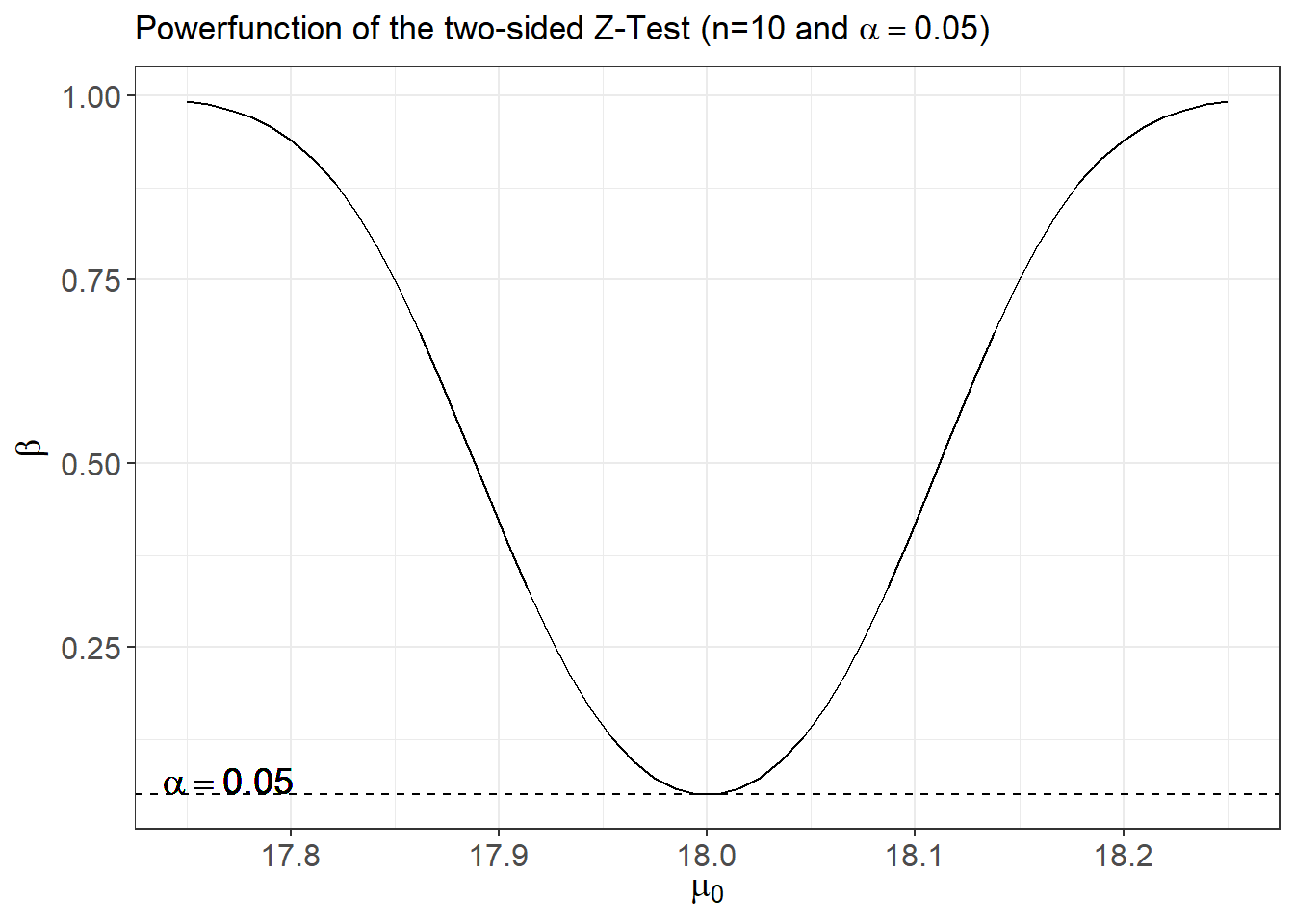

This example illustrates the power function of a sensible test, since:

Assuming that the basic assumptions (i.e., normality and known variance) are true, the above Gauss-test is the most prominent example of a uniformly most powerful test. Under its (restrictive) assumptions, no other possible test can achieve a larger value of $\beta_{n, \alpha}(\mu)$ for any possible value of $\mu$.

3.4 Asymptotic Null Distributions

Generally, the underlying distributions are unknown. In this case it is usually not possible to compute the power function of a test for fixed $n$. (Exceptions are so called “distribution-free” tests in nonparametric statistics.) The only way out of this difficulty is to rely on large sample asymptotics and corresponding asymptotic distributions, which allow to approximate the power function and to study the asymptotic efficiency of a test. The finite sample behavior of a test for different sample sizes $n$ is then evaluated by means of simulation studies.

For a real-valued parameter $\theta$ most tests of $H_{0}: \theta=\theta_{0}$ rely on estimators $\hat{\theta}$ of $\theta$. Under suitable regularity conditions on the underlying distribution, central limit theorems usually imply that $$\sqrt{n}(\hat{\theta}-\theta) \rightarrow^d N\left(0, v^{2}\right) \quad \text { as } \quad n \rightarrow \infty,$$ where $v^{2}$ is the asymptotic variance of the estimator.

Often a consistent estimator $\hat{v}^{2}$ of $v^{2}$ can be determined from the data. For large $n$ we then approximately have $$\frac{\sqrt{n}(\hat{\theta}-\theta)}{v} \stackrel{a}{\sim} N(0,1) .$$ For a given $\alpha$, a one-sided test of $H_{0}: \theta=\theta_{0}$ against $H_{1}: \theta>\theta_{0}$ then rejects $H_{0}$ if $$Z=\frac{\sqrt{n}\left(\hat{\theta}-\theta_{0}\right)}{v}>z_{1-\alpha} .$$ The corresponding asymptotic approximation (valid for sufficiently large $n$ ) of the true power function is then given by $$\beta_{n, \alpha}(\theta)=1-\Phi\left(z_{1-\alpha}-\frac{\sqrt{n}\left(\theta-\theta_{0}\right)}{v}\right)$$

Note that in practice the (unknown) true value $v^{2}$ is generally replaced by an estimator $\hat{v}^{2}$ determined from the data. As long as $\hat{v}^{2}$ is a consistent estimator of $v^{2}$ this leads to the same asymptotic power function. The resulting test is asymptotically unbiased and consistent.

Example Let $X_{1}, \ldots, X_{n}$ be an iid random sample. Consider testing $H_{0}: \mu=$ $\mu_{0}$ against $H_{1}: \mu>\mu_{0}$, where $\mu:=E\left(X_{i}\right)$. For a given level $\alpha$ the t-test then rejects $H_{0}$ if $$T=\frac{\sqrt{n}\left(\bar{X}-\mu_{0}\right)}{S}>t_{n-1 ; 1-\alpha},$$ where $t_{n-1 ; 1-\alpha}$ is the $1-\alpha$ quantile of a t-distributions with $(n-1)$-degrees of freedom. This is an exact test if the distribution of $X_{i}$ is normal.

In the general case, the justification of the t-test is based on asymptotic arguments. Under some regularity conditions the central limit theorem implies that $$\sqrt{n}(\bar{X}-\mu) \rightarrow^d N\left(0, \sigma^{2}\right) \quad \text { as } \quad n \rightarrow \infty$$ with $\sigma^{2}=\operatorname{Var}\left(X_{i}\right)$.

Moreover, $S^{2}$ is a consistent estimator of $\sigma^{2}$ and $t_{n-1 ; 1-\alpha} \rightarrow$ $z_{1-\alpha}$ as $n \rightarrow \infty$. Thus even if the distribution of $X_{i}$ is non-normal, for sufficiently large $n, T=\frac{\sqrt{n}\left(\bar{X}-\mu_{0}\right)}{S}$ is approximately $N(0,1)$-distributed and the asymptotic power function of the t-test is given by $$\beta_{n, \alpha}(\theta)=1-\Phi\left(z_{1-\alpha}-\frac{\sqrt{n}\left(\mu-\mu_{0}\right)}{\sigma}\right) .$$

3.5 Confidence Sets

Suppose we test $H_0: \theta = \theta_0$ and have a test such that $$P\left(T \in \mathcal C \mid H_0 \text{ is true} \right) = \alpha$$

Now collect all values of $\theta_0$ for which we do not reject the null hypothesis, and call this set $CS$. Then, $$P\left(\theta \in CS\right) = 1 - P\left(\theta \notin CS\right) = 1 - P\left(T \in \mathcal C \mid H_0 \text{ is true}\right) = 1 - \alpha$$

We call $CS$ an exact $1-\alpha$ confidence set for $\theta$.

Similarly, if $P\left(T \in \mathcal C \mid H_0 \text{ is true} \right) \rightarrow \alpha$, then $P\left(\theta \in CS\right) \rightarrow 1 - \alpha$ and $CS$ is an asymptotically valid $1-\alpha$ confidence set for $\theta$.

Example: In the previous example, we considered testing $H_{0}: \mu=$ $\mu_{0}$ against $H_{1}: \mu>\mu_{0}$, where $\mu:=E\left(X_{i}\right)$ using a random sample. For a given level $\alpha$ the t-test then rejects $H_{0}$ if $$T=\frac{\sqrt{n}\left(\bar{X}-\mu_{0}\right)}{S}>t_{n-1 ; 1-\alpha},$$ The corresponding confidence set is $$CS = \left\{ \mu \in \mathbb{R}: \bar{X} - t_{n-1 ; 1-\alpha} \frac{S}{\sqrt{n} } \leq \mu \leq \bar{X} + t_{n-1 ; 1-\alpha} \frac{S}{\sqrt{n} } \right\}$$ This is an exact confidence interval if we have a sample from a normal and an asymptotically valid confidence interval otherwise.