Chapter 4 Logistic regression models

Machine learning assumptions: (i) a dataset is available with observations for a number of explanatory X-variables and the corresponding value of a response Y-variable and (ii) there is a function f that describes the relationship between the X variables and the Y variable: Y = f(X1, X2,…, X3) + \(\epsilon\).

Machine Learning objective: to find the function f.

If the Y variable is categorical, we have a classification problem. The aim of constructing a model is to predict, given X values of new observations, the corresponding Y value. In other words to predict to which Y category the observation belongs. Models are usually constructed in such a way that the f-value per category gives a probability that the observation belongs to that category. The user of the model can then classify the observations himself based on these probabilities. This does not necessarily mean that the category with the highest probability is chosen. For example, if a doctor decides on the basis of observations that a patient has a 30% probability of having a certain disease, he may decide to prescribe drugs to combat this disease, although there is a 70% probability that this is unnecessary.

4.1 Binary Y-variable

If the Y-variable is dichotomous, i.e. has two categories, these are often labeled POS and NEG or 1 and 0 and sometimes -1 and +1. The latter is especially the case when a perceptron model is used to distinguish between the two Y-categories.

4.1.1 Linear regression with a binary Y-variable

If the Y-categories are labeled with the number 0 and 1, theoretical a regression model can be used, after all the Y-variable is numeric.
However, this method has some disadvantages:

assumptions of a linear regression model are violated
interpretation of predicted values; in a linear regression model, the model Y-value can be interpreted as the average Y-value, givena certain X-value; because the Y-variable is binary, an average Y-value given an X-value should be a value in the interval [0, 1] and can be interpreted as a probability; predicted values based on a linear regression model however, can be far outside this interval.

A model that can be used in case of a dichotomous Y variable, models the probabilities of Y=1 as a function of X: P (Y=1 | X) = f(X), where f is a function that only takes on values in the interval [0, 1]. An example of such a model is the widely used logistic regression model.

4.1.2 Logistic Regression Model

The simple logistic regression model:

P(Y=1 | X) = \(\frac{e^{\beta_0+\beta_1X}}{1+e^{\beta_0+\beta_1X}}\) or in short: P(X) = \(\frac{e^{\beta_0+\beta_1X}}{1+e^{\beta_0+\beta_1X}}\)
with e Euler’s number (2.7182…), known from mathematics.

The formula can be rewritten into: \(log(\frac{P(X)}{1-P(X)}) = \beta_0 + \beta_1X\)

The expression between the brackets has the form \(\frac{probability}{1-probability}\) which is known as an odds ratio.² A logistic regression model is also known as a log-odds-model or logit-model.

If this model is applied, the parameters of the model have to be estimated based on the observations in the training data. For this the so called maximum likelihood criterion is used.

Maximum Likelihood Criterion

Based on n observations for the X-variables, a logit model estimates the probabilities Y belongs to class 1, i.e. P(Y=1 | X).
Assume we have 5 observations, (X1, 1), (X2, 1), (X3, 1), (X4, 0), (X5, 0). Model probabilities are p1, p2, p3, p4, p5. For a model to be a good model, p1, p2 and p3 should be close to 1 and p4 and p5 close to 0.
The maximum likelihood criterion for choosing the best model is:
choose the model which maximizes p1 x p2 x p3 x (1-p4) x (1-p5).
This criterion can be easily generalized.

4.1.2.1 Example Logistic Regression Model

The example described in this section makes use of the Breast Cancer Wisconson Data Set, which can be found here.

library(tidyverse)
library(caret)
library(GGally) #vanwege ggpairs() plot
library(flextable)

df_read <- read_csv("Data/wbcd.csv")
df_read$id <- as.character(df_read$id)

Table
First Six Rows and Six Columns of the WBCD Data Set

flextable(head(df_read)[,1:6]) %>% autofit()

id	diagnosis	radius_mean	taxture_mean	perimeter_mean	area_mean
842302	M	18	10	123	1,001
842517	M	21	18	133	1,326
84300903	M	20	21	130	1,203
84348301	M	11	20	78	386
84358402	M	20	14	135	1,297
843786	M	12	16	83	477

The first column is a unique identifier, the second column - diagnosis - is the target variable. Thw data set contains 30 X-variables. In this example only the first six X-variables are taken into account.

Figure
Summary of the WBCD Data Set

df <- df_read[,2:8]
summary(df)

  diagnosis          radius_mean      taxture_mean   perimeter_mean  
 Length:569         Min.   : 6.981   Min.   : 9.71   Min.   : 43.79  
 Class :character   1st Qu.:11.700   1st Qu.:16.17   1st Qu.: 75.17  
 Mode  :character   Median :13.370   Median :18.84   Median : 86.24  
                    Mean   :14.127   Mean   :19.29   Mean   : 91.97  
                    3rd Qu.:15.780   3rd Qu.:21.80   3rd Qu.:104.10  
                    Max.   :28.110   Max.   :39.28   Max.   :188.50  
   area_mean      smoothness_mean   compactness_mean 
 Min.   : 143.5   Min.   :0.05263   Min.   :0.01938  
 1st Qu.: 420.3   1st Qu.:0.08637   1st Qu.:0.06492  
 Median : 551.1   Median :0.09587   Median :0.09263  
 Mean   : 654.9   Mean   :0.09636   Mean   :0.10434  
 3rd Qu.: 782.7   3rd Qu.:0.10530   3rd Qu.:0.13040  
 Max.   :2501.0   Max.   :0.16340   Max.   :0.34540

Note. Only 6 of the 30 available X-variables are used in the example and summarized in this overview.

The diagnosis-variable is transformed into a factor variable. The GGally::ggpairs() function is used to examine the correlation between the different variables.

Figure
Correlation Plot Matrix

df$diagnosis <- factor(df$diagnosis,
                       levels=c("B", "M"),
                       labels=c("NEG", "POS"))
ggpairs(df)

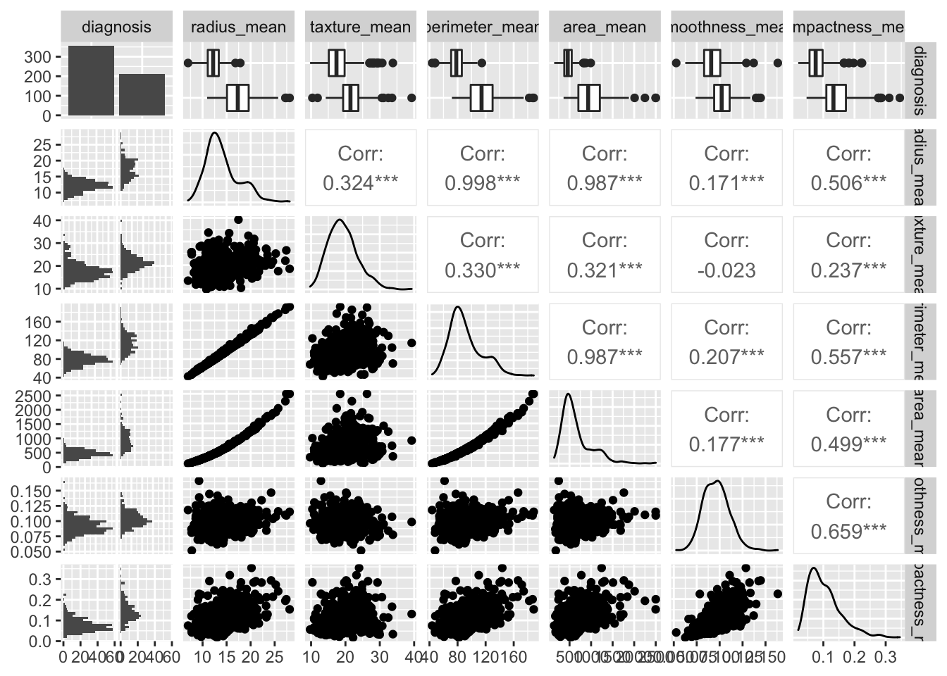The area_mean variable seems to make a good candidate to distinguish diagnosis M from diagnosis B.
The first logistic regression model usus this variable as the only predictor.

logreg_model1 <- glm(diagnosis~area_mean, data = df,
                     family = "binomial")
preds_logreg1 <- predict(logreg_model1, type = 'response')

threshold <- .5
preds_logreg1_diag <- ifelse(preds_logreg1>.5, "POS", "NEG") %>% 
  factor()
         
confusionMatrix(preds_logreg1_diag, df$diagnosis,
                positive = "POS")

Confusion Matrix and Statistics

          Reference
Prediction NEG POS
       NEG 337  46
       POS  20 166
                                          
               Accuracy : 0.884           
                 95% CI : (0.8548, 0.9091)
    No Information Rate : 0.6274          
    P-Value [Acc > NIR] : < 2.2e-16       
                                          
                  Kappa : 0.7456          
                                          
 Mcnemar's Test P-Value : 0.002089        
                                          
            Sensitivity : 0.7830          
            Specificity : 0.9440          
         Pos Pred Value : 0.8925          
         Neg Pred Value : 0.8799          
             Prevalence : 0.3726          
         Detection Rate : 0.2917          
   Detection Prevalence : 0.3269          
      Balanced Accuracy : 0.8635          
                                          
       'Positive' Class : POS

library(tidyverse)

## ── Attaching packages ─────────────────────────────────────── tidyverse 1.3.0 ──

## ✓ ggplot2 3.3.3     ✓ purrr   0.3.4
## ✓ tibble  3.0.4     ✓ dplyr   1.0.2
## ✓ tidyr   1.1.2     ✓ stringr 1.4.0
## ✓ readr   1.4.0     ✓ forcats 0.5.0

## ── Conflicts ────────────────────────────────────────── tidyverse_conflicts() ──
## x dplyr::filter() masks stats::filter()
## x dplyr::lag()    masks stats::lag()

library(rpart)
library(rpart.plot)
library(caret)

## Loading required package: lattice

## 
## Attaching package: 'caret'

## The following object is masked from 'package:purrr':
## 
##     lift

library(flextable)

## 
## Attaching package: 'flextable'

## The following object is masked from 'package:purrr':
## 
##     compose

if the probability of a particular event equals 1/6, then the odds ratio equals 1/5 or 1 against 5; the probability that the event will not occur is 5 times higher than that it will occur. If for a particular event the odd ratio equals 4 (4 against 1), then the probability the event happens is 4/5 (80%).↩︎