Chapter 3 Linear regression models

3.1 Simple linear regression

A simple linear regression model describes the relation between a numeric Y-variable and one numeric X-variable with a linear equation. The general form is:

\(Y = \beta_0 + \beta_1X + \epsilon\) with:

\(\beta_0\) the intercept
\(\beta_1\) the slope
\(\epsilon\) the residual or error term; this term stands for the effect of other variables on Y and for random variation in the Y-variable

Applying this model on a data set means estimating the values of the model parameters, \(\beta_0\) and \(\beta_1\), based on the available data.

3.1.1 Assessing a simple linear regression model

To assess the usefulness of an estimated regression model we use the coefficient of determination, R squared, the significance of the relationship between the Y- and the X-variable and the MSE (Mean Squared Error) or the Root Mean Squared Error (RMSE).

3.1.2 R squared (\(R^2\))

The coefficient of determination, \(R^2\), equals 1 minus the quotient of the variation of the Y-values around the regression line and the total variation in the Y-values.

\(R^2 = 1-\frac{\sum(Y-\hat{Y})^2}{\sum(Y-\bar{Y})^2} = 1 - \frac{\sum e_i^2}{\sum(Y-\bar{Y})^2}\)

The numerator in the fraction in these formulas, \(\sum e_i^2\), measures the variation in the Y-values which is not explained by the regression model. The denominator, \(\sum(Y-\bar{Y})^2\), measures the total variation in the Y-values. So the fraction measures the proportion of unexplained variation in the Y-values; 1 minus this fraction measures the proportion of the variation in the Y-values which is explained by the regression model.

For instance, if \(R^2\) = .65, 65% of the variation in the Y-values is explained by the model; in other words, 65% of the variation in the Y-values can be explained by the variation in the X-values.

3.1.3 Significance of the X-variable in the model

Another way to assess a regression model is testing the significance of the coefficient of the X-variable. This is done by testing H_A_: \(\beta_1 \neq 0\). If no support is found in the data for this hypothesis, the X-variable is not a significant variable. Or in other words, the Y-variable doesn’t depend significantly on the X-variable. Software packages used to generate a linear regression model, will also report the p-value for this test. A p-value below .05 is commonly interpreted as a significant result.

3.1.4 Mean Squared Error and Root Mean Squared Error

The most used metric to assess a regression model is the MSE (Mean Squared Error) or the square root of the MSE, the RMSE (Root Mean Squared Error):
\(MSE = \frac{\sum e_i^2}{N}\)
\(RMSE = \sqrt{\frac{\sum e_i^2}{N}}\)
These metrics measure the average distance of the data points to the regression line, measured in the Y direction. It is a metric which measures the model error.

Remember that in general we are more interested in the out-of-sample performance than in the in-sample performance. In case of a (simple) linear regression model, it can be shown that the in-sample MSE is a good estimate for the out-of-sample MSE. The estimate can even be improved by using N-2 in the denominator in stead of N:
\(RMSE = \sqrt{\frac{\sum e_i^2}{N-2}}\).

Of course the commonly used techniques to estimate the out of sample error can be used as wel, such as splitting the data set in a training and a test set, cross validation or bootstrapping. In the example in the next session the different techniques to estimate the out-of-sample performance of a linear rergession model are illustrated, using an example.

3.2 Example simple linear regression

As an example of applying a linear regression model, we use a dataset with a random sample of Dutch cars from three brands: AUDI, CITROEN and KIA. The data is sampled from the RDW website on August 20, 2020. Data from two databases on this website are joined into one data frame and some data cleaning has been performed.

Table 3.1
First 10 Observations in RDW Data Set

library(tidyverse)
library(flextable)
library(kableExtra)
rdw_sample <- read_csv("data/20200820rdw_sample.csv")
flextable(head(rdw_sample, n = 10)) %>% fontsize(size = 7, part = "all")

Figure 3.1
Summary of the RDW Dataset

summary(rdw_sample)

 LICENSE_PLATE         BRAND              COLOR           ECONOMY_LABEL     
 Length:8341        Length:8341        Length:8341        Length:8341       
 Class :character   Class :character   Class :character   Class :character  
 Mode  :character   Mode  :character   Mode  :character   Mode  :character  
                                                                            
                                                                            
                                                                            
 FUEL_DESCRIPTION   CILINDER_CONTENT      MASS      CATALOG_PRICE  
 Length:8341        Min.   : 998     Min.   : 765   Min.   : 2423  
 Class :character   1st Qu.:1197     1st Qu.: 989   1st Qu.:17485  
 Mode  :character   Median :1396     Median :1215   Median :25750  
                    Mean   :1472     Mean   :1202   Mean   :29271  
                    3rd Qu.:1598     3rd Qu.:1402   3rd Qu.:35980  
                    Max.   :4163     Max.   :2420   Max.   :99983  
  SPECIAL_TAX   
 Min.   :    9  
 1st Qu.: 1573  
 Median : 3084  
 Mean   : 4102  
 3rd Qu.: 5662  
 Max.   :27622  

The aim is to generate a model that estimates the Catalogue Price (CATALOG_PRICE) given the value of the other variables as predictors, excepted the Special Tax variable (this variable cannot be a predictor for the catalogue price, because this special tax depends on this price).

The first model is a simple linear model with MASS as predictor for CATALOG_PRICE.

Figure 3.2
Output Simple Linear Regression Model in R

library(MOTE) #apa() function for apa representation of numbers

linmod_01 <- lm(CATALOG_PRICE ~ MASS, data = rdw_sample)
Rsquared <- apa(summary(linmod_01)$r.squared, 3, FALSE)
rmse <- prettyNum(round(summary(linmod_01)$sigma, 0), big.mark = ",")
mse <- prettyNum(summary(linmod_01)$sigma^2, big.mark = ",")
summary(linmod_01)

Call:
lm(formula = CATALOG_PRICE ~ MASS, data = rdw_sample)

Residuals:
   Min     1Q Median     3Q    Max 
-45568  -5890    475   3837  48936 

Coefficients:
              Estimate Std. Error t value Pr(>|t|)    
(Intercept) -3.125e+04  4.434e+02  -70.47   <2e-16 ***
MASS         5.033e+01  3.599e-01  139.85   <2e-16 ***
---
Signif. codes:  0 '***' 0.001 '**' 0.01 '*' 0.05 '.' 0.1 ' ' 1

Residual standard error: 8833 on 8339 degrees of freedom
Multiple R-squared:  0.7011,    Adjusted R-squared:  0.701 
F-statistic: 1.956e+04 on 1 and 8339 DF,  p-value: < 2.2e-16

In the output can be seen that \(R^2\) = .701; in other words 70.1% of the variation in the catalog prices is explained by the model.
MASS is a significant variable in the model, P-value < .001. The RMSE, in the output named as ‘Residual standard error’, equals 8,833. The MSE is just this number squared, MSE = 78,020,205.

As said before, in case of a (simple) linear regression model, the so calculated MSE is a good estimate for the out-of-sample MSE. This is the case, because with a linear regression model, possible overfitting is not really an issue. However, for more complicated models, it is.
To explain the concepts for estimating out-of-sample errors when using more complex models, in the next seections the MSE is calculated in more general ways.

3.2.1 Estimating out-of-sample error using a training and a test set

The first method splits the data randomly in a training set and a test set. The model parameters are estimated using the training set. The out-of-sample error is estimated using the test set.

set.seed(20200823)
prop_train <- .50
train <- sample(1:nrow(rdw_sample), prop_train*nrow(rdw_sample))
rdw_train <- rdw_sample[train,]
rdw_test <- rdw_sample[-train,]

linmod_02 <- lm(CATALOG_PRICE ~ MASS, data = rdw_train)
predict_train <- predict(linmod_02)
MSE_train <- sum((predict_train - rdw_train$CATALOG_PRICE)^2)/(nrow(rdw_train) - 2)
RMSE_train <- prettyNum(sqrt(MSE_train),
                        digits=0,
                        big.mark = ",")
#alternative
#RMSE_train <- summary(linmod_02)$sigma

predict_test <- predict(linmod_02, newdata = rdw_test)
MSE_test <- mean((predict_test - rdw_test$CATALOG_PRICE)^2)
RMSE_test <- prettyNum(sqrt(MSE_test), 
                       digits=0, big.mark = ",")

The within sample RMSE, i.e. the RMSE calculated based on the training data, equals 8,673. The out-of-sample error estimate equals 8,992.

3.2.2 Estimating out-of-sample error using cross validation

In this section 10-fold cross validation is used to estimate the out-of-sample RMSE.

#10-fold CV
library(caret)
library(tidyverse)
library(kableExtra)
set.seed(20200824)
rdw_sample$GROUP <- sample(c(1, rep(1:10, 834)))

MSEs <- NULL

for (t in 1:10) {
  trainset <- filter(rdw_sample, GROUP != t)
  testset <- filter(rdw_sample, GROUP == t)
  linmod <- lm(CATALOG_PRICE ~ MASS, data = trainset)
  predict_test <- predict(linmod, newdata = testset)
  mse <- mean((predict_test - testset$CATALOG_PRICE)^2)
  MSEs[t] = mse
}
mse_estimate <- mean(MSEs)
rmse_estimate <- sqrt(mse_estimate)

This procedure leads to 10 estimates for the out-of-sample MSE: 72,139,107, 71,120,651, 78,852,650, 74,810,525, 71,190,694, 77,776,460, 77,709,740, 84,458,930, 84,033,745, 88,307,401. The average of these estimates, 78,039,990, is the CV estimate of the out-of-sample MSE. The RMSE estimate is 8,834.
The variation in the estimates can be used to make a statement about the accuracy of the CV estimate, or to calculate an interval estimate for the out-of-sample error. To improve such an interval estimate, the CV procedure can be repeated dozens or hundreds of times; if this is done this procedure is called Repeated Cross Validation. For instance, if the procedure is repeated 200 times, this leads to 2000 estimates for the out-of-sample MSE, which can be used to calculate an interval estimate for the out-of-sample estimate. To calculate a 95% confidence interval (CI) for the out-of-smaple MSE, the .025th and the .975th quantile of the 2000 estimates are calculated. The probability that the interval between these two values contains the “real” out-of-sample MSE equals 95%.

#200 times repeated 10-fold CV
set.seed(20200829)

MSEs <- NULL

for (i in 1:200) {
rdw_sample$GROUP <- sample(c(1, rep(1:10, 834)))
for (t in 1:10) {
  trainset <- filter(rdw_sample, GROUP != t)
  testset <- filter(rdw_sample, GROUP == t)
  linmod <- lm(CATALOG_PRICE ~ MASS, data = trainset)
  predict_test <- predict(linmod, newdata = testset)
  mse <- mean((predict_test - testset$CATALOG_PRICE)^2)
  MSEs <- c(MSEs, mse)
}}

RMSEs <- sqrt(MSEs)
mse_estimate <- mean(MSEs)
mse_estimate_025 <- quantile(MSEs, .025)
mse_estimate_975 <- quantile(MSEs, .975)
rmse_estimate <- mean(sqrt(MSEs))
rmse_estimate_025 <- quantile(sqrt(MSEs), .025)
rmse_estimate_975 <- quantile(sqrt(MSEs), .975)


rmse_plot <- tibble(RMSE = RMSEs) %>%
  ggplot(aes(x=RMSE)) + 
  geom_histogram(binwidth = 50, fill = "royalblue") +
  geom_vline(aes(xintercept = rmse_estimate_025), col = "grey") +
  geom_vline(aes(xintercept = rmse_estimate_975), col = "grey") +
  theme_minimal()

Figure 3.3
RMSE Estimates Based on 200 times Repeated 10-folds CV

rmse_plot

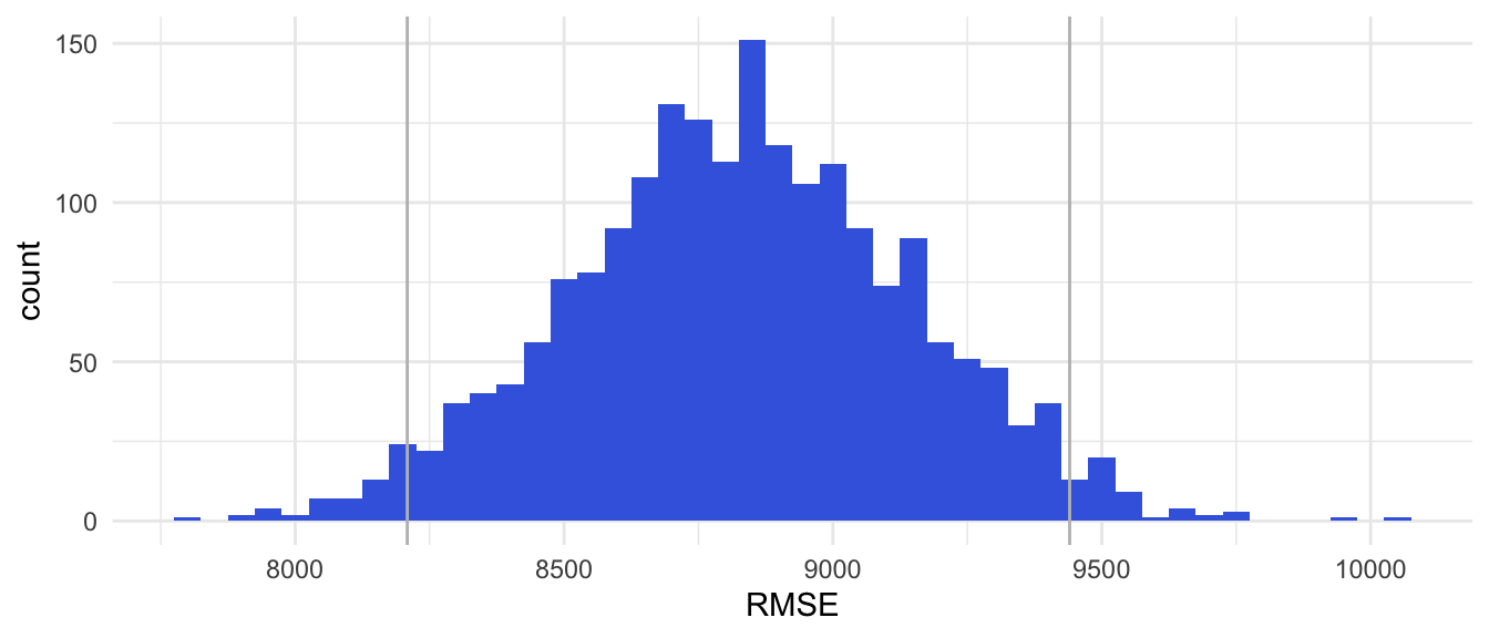
Figure 3.1: rmse_plot

Note. The gray lines mark the 95% CI for the RMSE.

In this example 200 times Repeated 10-fold CV, leads to:
point estimate for the out-of-sample MSE: 78,060,204
point estimate for the out-of-sample RMSE: 8,830
95% interval estimate for out-of-sample MSE: <67,379,651; 89,119,641>
95% interval estimate for out-of-sample RMSE: <8,209; 9,440>.

3.2.3 Estimating out-of-sample-error using bootstrapping

Bootstrapping is a technique of resampling from the available data set. Hundreds or even thousands of samples from the data set are drawn wtih replacement and sample size the number of observartions in the data set. This means that observations can be drwan more than one time in a bootstrap sample.
Bootstrapping is based on just one assumption: the available data form a representative sample of the research population. Under this assumption the population can be assumed to consist of a couple of thousand times this sample. Drawing a sample from this assumed population, is the same as drawing a sample from the available sample data with replacement. Bootstrap samples have the same sample size as the originale available sample data set. Under the mentioned assumption, a bootstrap sample can be seen as a random sample from the population of interest. Drawing 200 bootstrap samples yields 200 possible samples from the research population. These bootstrap samples can be used to estimate unknown population parameters, e.g. an MSE in a simple linear regression problem.

#200 bootstrap samples
set.seed(20200829)
MSEs_bootstrap <- NULL
for (i in 1:200) {
  sample <- sample_n(rdw_sample, size = nrow(rdw_sample),replace = TRUE)
  linmod <- lm(CATALOG_PRICE~MASS, data = sample)
  predict_bootstrap <- predict(linmod)
  mse <- mean((predict_bootstrap - sample$CATALOG_PRICE)^2)
  MSEs_bootstrap <- c(MSEs_bootstrap, mse)
}

RMSEs_bootstrap <- sqrt(MSEs_bootstrap)

rmse_bootstrap_plot <- tibble(RMSE = RMSEs_bootstrap) %>%
  ggplot(aes(x=RMSE)) + 
  geom_histogram(binwidth = 50, fill = "royalblue") +
  geom_vline(aes(xintercept = quantile(RMSEs_bootstrap, .025)), col = "grey") +
  geom_vline(aes(xintercept = quantile(RMSEs_bootstrap, .975)), col = "grey") +
  theme_minimal()

Figure 3.4
RMSE estimates based on 200 Bootstrap Samples

rmse_bootstrap_plot

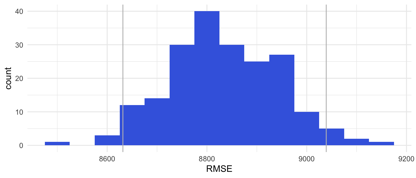
Results bootstrap sampling
Estimate out-of-sample MSE = 78,056,696
Estimate out-of-sample RMSE = 8,834

3.3 Caret Package

The caret package is a usefull R package to apply a Machine Learning (ML) model on a data set. Actually it is not one package, but a combination of dozens of packages which are developed for all kinds of different ML models. The central function to apply a ML model on a sample is the train() function. This section provides the code when using the caret package, for the examples in the former sections.

3.3.1 Estimating MSE using bootstrap

The first example is the use of the bootstrap sampling method. The reason for starting with the bootstrap sample, is because this is the default method in the caret package.

Figure 3.5
The Generated Linear Model with Caret, Default Settings

library(caret)
set.seed(20200829)
linmod_caret_bootstrap <-
  train(CATALOG_PRICE~MASS, data = rdw_sample, method = "lm")

linmod_caret_bootstrap

Linear Regression 

8341 samples
   1 predictor

No pre-processing
Resampling: Bootstrapped (25 reps) 
Summary of sample sizes: 8341, 8341, 8341, 8341, 8341, 8341, ... 
Resampling results:

  RMSE      Rsquared   MAE   
  8815.187  0.7015241  6444.3

Tuning parameter 'intercept' was held constant at a value of TRUE

Examine the output in Table 3.1 carefully to understand how the caret package generates a linear model. As default caret produces 25 bootstrap samples to estimate the out-of-sample performance. The reported out-of-sample error is the average of 25 estimated out-of-sample errors. The reported RMSE is the bootstrap RMSE, the square root of the average of 25 bootstrapped MSE’s.

Figure 3.6
The Summary of the Linear Model

summary(linmod_caret_bootstrap)

Call:
lm(formula = .outcome ~ ., data = dat)

Residuals:
   Min     1Q Median     3Q    Max 
-45568  -5890    475   3837  48936 

Coefficients:
              Estimate Std. Error t value Pr(>|t|)    
(Intercept) -3.125e+04  4.434e+02  -70.47   <2e-16 ***
MASS         5.033e+01  3.599e-01  139.85   <2e-16 ***
---
Signif. codes:  0 '***' 0.001 '**' 0.01 '*' 0.05 '.' 0.1 ' ' 1

Residual standard error: 8833 on 8339 degrees of freedom
Multiple R-squared:  0.7011,    Adjusted R-squared:  0.701 
F-statistic: 1.956e+04 on 1 and 8339 DF,  p-value: < 2.2e-16

Table 3.2 shows the model that is reported as the final model. This final model is based on all available data. This model will be used if predictions for new data are made with the bootstrap model.

In the default setting 25 bootstrap samples are used to estimate the out-of-sample performance. With the trControl argument of the train() function, this number can be adjusted to another number.

Figure 3.7
Caret Linear Model Based on 200 Bootstrap Samples

library(caret)
set.seed(20200829)
linmod_caret_bootstrap_200 <-
  train(CATALOG_PRICE~MASS, data = rdw_sample, method = "lm",
        trControl = trainControl(number = 200))
linmod_caret_bootstrap_200

Linear Regression 

8341 samples
   1 predictor

No pre-processing
Resampling: Bootstrapped (200 reps) 
Summary of sample sizes: 8341, 8341, 8341, 8341, 8341, 8341, ... 
Resampling results:

  RMSE      Rsquared   MAE     
  8834.139  0.7017922  6455.909

Tuning parameter 'intercept' was held constant at a value of TRUE

The summary of this model is based on all the observations in the training set and is the same as the model in Figure 3.2.

Figure 3.8
Summary Caret Linear Model Based on 200 Bootstrap Samples

summary(linmod_caret_bootstrap_200)

Call:
lm(formula = .outcome ~ ., data = dat)

Residuals:
   Min     1Q Median     3Q    Max 
-45568  -5890    475   3837  48936 

Coefficients:
              Estimate Std. Error t value Pr(>|t|)    
(Intercept) -3.125e+04  4.434e+02  -70.47   <2e-16 ***
MASS         5.033e+01  3.599e-01  139.85   <2e-16 ***
---
Signif. codes:  0 '***' 0.001 '**' 0.01 '*' 0.05 '.' 0.1 ' ' 1

Residual standard error: 8833 on 8339 degrees of freedom
Multiple R-squared:  0.7011,    Adjusted R-squared:  0.701 
F-statistic: 1.956e+04 on 1 and 8339 DF,  p-value: < 2.2e-16

3.3.2 Estimating MSE using Repeated Cross Validation

The trControl() argument in the caret::train() funciton can also be used to use another method for estimating the out-of-sample performance. For instance cross validation or repeated cross validation.

Figure 3.8
Caret Linear Model Based on 200 Times Repeated 10-Fold CV

set.seed(20200829)
linmod_caret_repeatedcv <-
  train(CATALOG_PRICE~MASS, data = rdw_sample, method = "lm",
        trControl = trainControl(method="repeatedcv", number=10,
                                 repeats = 200))
linmod_caret_repeatedcv

Linear Regression 

8341 samples
   1 predictor

No pre-processing
Resampling: Cross-Validated (10 fold, repeated 200 times) 
Summary of sample sizes: 7506, 7508, 7506, 7508, 7508, 7507, ... 
Resampling results:

  RMSE      Rsquared   MAE     
  8828.989  0.7015469  6460.448

Tuning parameter 'intercept' was held constant at a value of TRUE

Figure 3.9
Summary Caret Linear Model Based on 200 Times Repeated 10-Fold CV

summary(linmod_caret_repeatedcv)

Call:
lm(formula = .outcome ~ ., data = dat)

Residuals:
   Min     1Q Median     3Q    Max 
-45568  -5890    475   3837  48936 

Coefficients:
              Estimate Std. Error t value Pr(>|t|)    
(Intercept) -3.125e+04  4.434e+02  -70.47   <2e-16 ***
MASS         5.033e+01  3.599e-01  139.85   <2e-16 ***
---
Signif. codes:  0 '***' 0.001 '**' 0.01 '*' 0.05 '.' 0.1 ' ' 1

Residual standard error: 8833 on 8339 degrees of freedom
Multiple R-squared:  0.7011,    Adjusted R-squared:  0.701 
F-statistic: 1.956e+04 on 1 and 8339 DF,  p-value: < 2.2e-16

The output of the train() function is a list with lots of information. One of the components of the list is the ‘results’ component. Besides the estimated RMSE and R squared value.

Figure 3.10
Results Caret Linear Model Based on 200 Times Repeated 10-Fold CV

linmod_caret_repeatedcv$results

  intercept     RMSE  Rsquared      MAE RMSESD RsquaredSD    MAESD
1      TRUE 8828.989 0.7015469 6460.448 302.76 0.01411291 180.9893

If 200 times repeated 10-Fold CV is applied, 2000 linear models are generated and evaluated. The reported out-of-sample performance is the average of 2000 out-of-sample performance estimates. The reported standard deviation (RMSESD) is the standard deviation of these 2000 estimates.