Chapter 5 Classification Decision Trees
Decision Trees are probably the most basic models for classification problems. Many websites with an introduction to Decision Trees can be found on the internet, see for instance this website.
5.1 Splitting Criteria
The question what the best choice for a node, i.e. a variable and a splitting criterion, requires a metric to measure how good a possible split is. Commonly choices are (1) Information Gain and (2) Gini Impurity. Another possibility, which was widely used in the past, uses a Chi-Square Criterion.
The concepts are discussed in the next sub sections.
5.1.1 Measuring Information Gain
5.1.2 Gini Impurity
5.1.3 Chi-Square Criterion
Probably the oldest splitting criterion used when generating a decision tree makes uses of Chi-Square statitics to find out which of the features is strongest correlated to the target function.
However it is no longer used that often, and is beyond the scope of this book.
5.2 Example: Predicting Diabetes
Predicting diabetes
Data set: example from UCI website
The data set consists of 520 observations on 17 features. The target variable is the Class variable which can take on two values, Positive and Negative. All but one of the features are binary. The non binary feature is the Age feature.
Table 1
First Six Observations of the Diabetes Data Set
Age | Gender | Polyuria | Polydipsia | sudden weight loss | weakness | Polyphagia | Genital thrush | visual blurring | Itching | Irritability | delayed healing | partial paresis | muscle stiffness | Alopecia | Obesity | class |
40 | Male | No | Yes | No | Yes | No | No | No | Yes | No | Yes | No | Yes | Yes | Yes | Positive |
58 | Male | No | No | No | Yes | No | No | Yes | No | No | No | Yes | No | Yes | No | Positive |
41 | Male | Yes | No | No | Yes | Yes | No | No | Yes | No | Yes | No | Yes | Yes | No | Positive |
45 | Male | No | No | Yes | Yes | Yes | Yes | No | Yes | No | Yes | No | No | No | No | Positive |
60 | Male | Yes | Yes | Yes | Yes | Yes | No | Yes | Yes | Yes | Yes | Yes | Yes | Yes | Yes | Positive |
55 | Male | Yes | Yes | No | Yes | Yes | No | Yes | Yes | No | Yes | No | Yes | Yes | Yes | Positive |
Table 2
Summary of the data
summary(df)
##       Age           Gender            Polyuria          Polydipsia
##  Min.   :16.00   Length:520         Length:520         Length:520
##  1st Qu.:39.00   Class :character   Class :character   Class :character
##  Median :47.50   Mode  :character   Mode  :character   Mode  :character
##  Mean   :48.03
##  3rd Qu.:57.00
##  Max.   :90.00
##  sudden weight loss   weakness          Polyphagia        Genital thrush
##  Length:520         Length:520         Length:520         Length:520
##  Class :character   Class :character   Class :character   Class :character
##  Mode  :character   Mode  :character   Mode  :character   Mode  :character
##
##
##
##  visual blurring      Itching          Irritability       delayed healing
##  Length:520         Length:520         Length:520         Length:520
##  Class :character   Class :character   Class :character   Class :character
##  Mode  :character   Mode  :character   Mode  :character   Mode  :character
##
##
##
##  partial paresis    muscle stiffness     Alopecia           Obesity
##  Length:520         Length:520         Length:520         Length:520
##  Class :character   Class :character   Class :character   Class :character
##  Mode  :character   Mode  :character   Mode  :character   Mode  :character
##
##
##
##     class
##  Length:520
##  Class :character
##  Mode  :character
##
##
##
Data cleaning and Preprocessing
Correct variable names (no spaces).
Transform class variable in a factor variable with two levels, POS and NEG.
5.2.0.1 Creating a Decision Tree Model using Rpart
As a first step, split the data set in a training and a test set; 70% in training, 30% in test set (other choices are possible as well). The caret::createDataPartition() function, can be used to create a partition such that the proportion Positives and Negatives are the same in the training and in the test set, a so called stratified sample.
#split in training end test set
set.seed(20210309)
train <- createDataPartition(df_prep$CLASS, p=0.70, list=FALSE)
df_train <- df_prep[train,]
## Warning: The `i` argument of ``[`()` can't be a matrix as of tibble 3.0.0.
## Convert to a vector.
## This warning is displayed once every 8 hours.
## Call `lifecycle::last_warnings()` to see where this warning was generated.Use rpart::rpart() to create a decision tree.
This funciton uses Gini as default to measure impurity and information gain as alternative option.
See https://www.rdocumentation.org/packages/rpart/versions/4.1-15/topics/rpart
In this example, Accuracy is used as metric to assess the decision tree.
Create decision tree.
tree_01 <- rpart(CLASS~., data = df_train)

#other option
#tree_01 <- rpart(CLASS~., data = df_train,
#                 parms = list(split = "gini"))
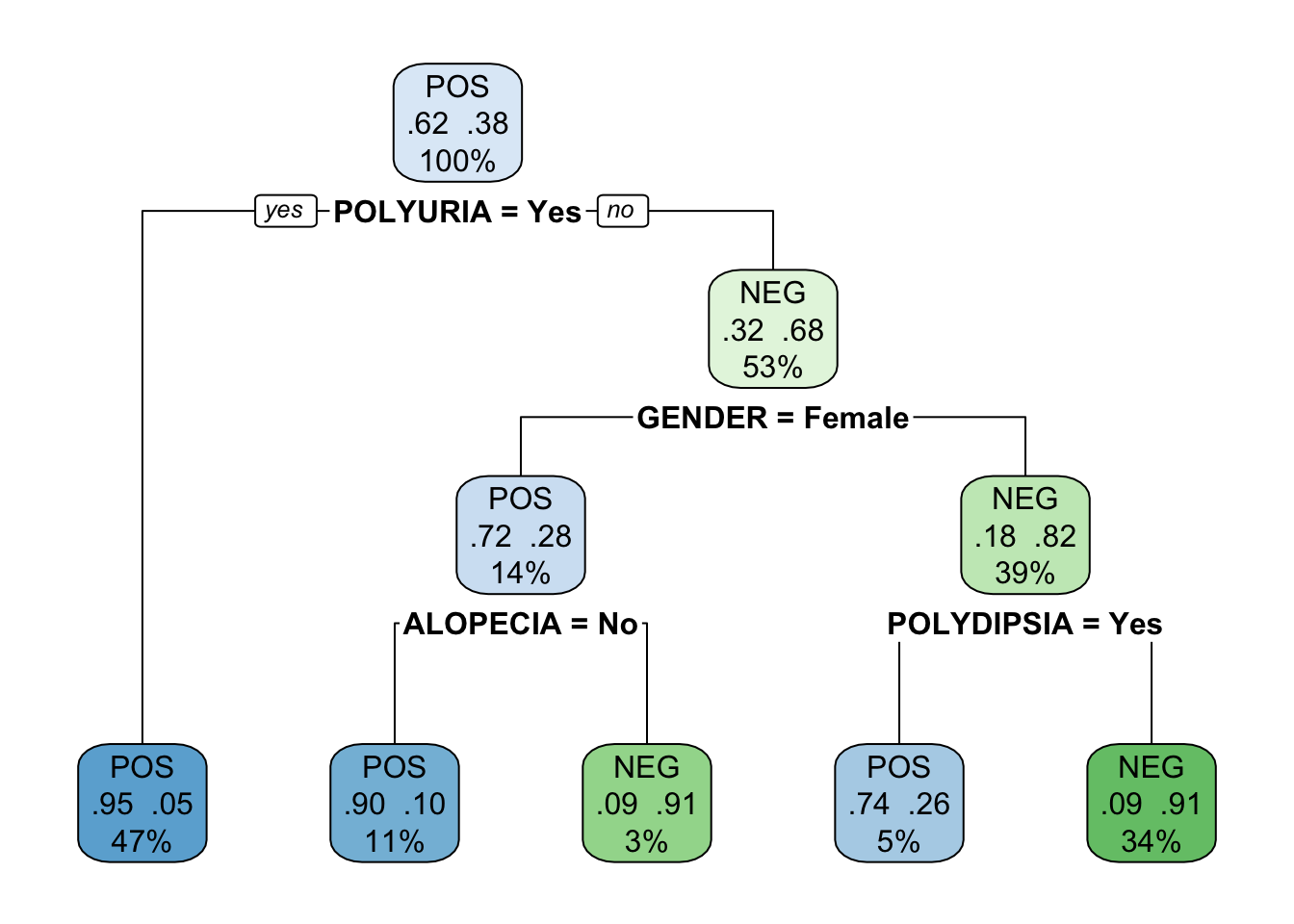
Plot the decision tree using rpart.plot::rpart.plot() function.
## Loading required package: rpart
This is the default tree plot made bij the rpart.plot() function. Each node shows (1) the predicted class, (2) the predicted probability of NEG and (3) the percentage of observations in the node. It is possible to change the lay-out of the plots and/or to show other information in the nodes.
For more information about the rpart.plot() function, see the help function and the vignette.
#### Assessing the decision tree model {-}
First assess the model on the training data:
- use predict() function to make predictions with the tree_01 model
- construct a confusion matrix
- calculate model Accuracy
Table 1
Confusion Matrrix Tree Model on Training Data
preds_tree01 <- predict(tree_01, newdata = df_train, type = 'class')
cm <- table(preds_tree01, df_train$CLASS)
cm
preds_tree01 POS NEG
         POS 212  18
         NEG  12 122
The Accuracy on the training data equals 0.918. This is a very high Accuracy, but the Accuracy on the test set is more interesting.
Table 2
Confusion Matrrix Tree Model on Test Data
preds_tree01 <- predict(tree_01, newdata = df_test, type = 'class')
cm_test <- table(preds_tree01, df_test$CLASS)
cm_test
preds_tree01 POS NEG
         POS  92  11
         NEG   4  49
The Accuracy on the test data equals 0.904. Although it is a bit lower than the Accuracy on the training data, it is still a high Accuracy.
It seems that the decision tree model performs quit well on this dataset.
The Accuracy on the test data is the estimate for the performance of the model outside the data used to construct the model. This estimates highly depends on the splitting in a training and a test set. Another split could lead to a different estimate. That’s why repeating this procedure and using the average of the estimates for the Accuracy as the estimate for the out-of-sample Accuracy is recommended. Cross Validation or Bootstrapping are other options to come to a good estimate for the out-of-sample performance of the model.
The R caret package has built-in possibilities to use one of these techniques to assess the performance of a ML model.
5.2.0.2 Creating a Decision Tree Model using Rpart within caret package
In this section the caret package is used to generate an rpart decision tree model.
The central function in the caret package is the train() function. It can be used to generate a wide variety of models. Actually the caret package is a package which includes a variety of packages to generate ML models. Besides that it provides preprocessing functions and options to use cross validation, bootstrapping, splitting data in training and test data and lots more.
First explore the use of rpart with default settings for most of the options provided.
Table 3
Decision Tree with rpart Method in Caret
CART

520 samples
 16 predictor
  2 classes: 'POS', 'NEG'

No pre-processing
Resampling: Bootstrapped (25 reps)
Summary of sample sizes: 520, 520, 520, 520, 520, 520, ...
Resampling results across tuning parameters:

  cp     Accuracy   Kappa
  0.060  0.8661589  0.7171642
  0.125  0.8260738  0.6477010
  0.540  0.7351813  0.4029460

Accuracy was used to select the optimal model using the largest value.
The final value used for the model was cp = 0.06.
Points of attention:
- splitting in training and test data is done by the functions within caret; caret uses 25 times repeated bootstrapping as default method to estimate the performance of the generated model
- caret uses a tuning parameter (cp, complexity parameter) to decide about tree depth; for more information see: ….. ; three different values are tested, for the final model the value with the best performance is used; so actually the total number of decision trees generated equals 75, 25 for each value of the tuning parameter
5.2.0.3 Plotting the decision tree
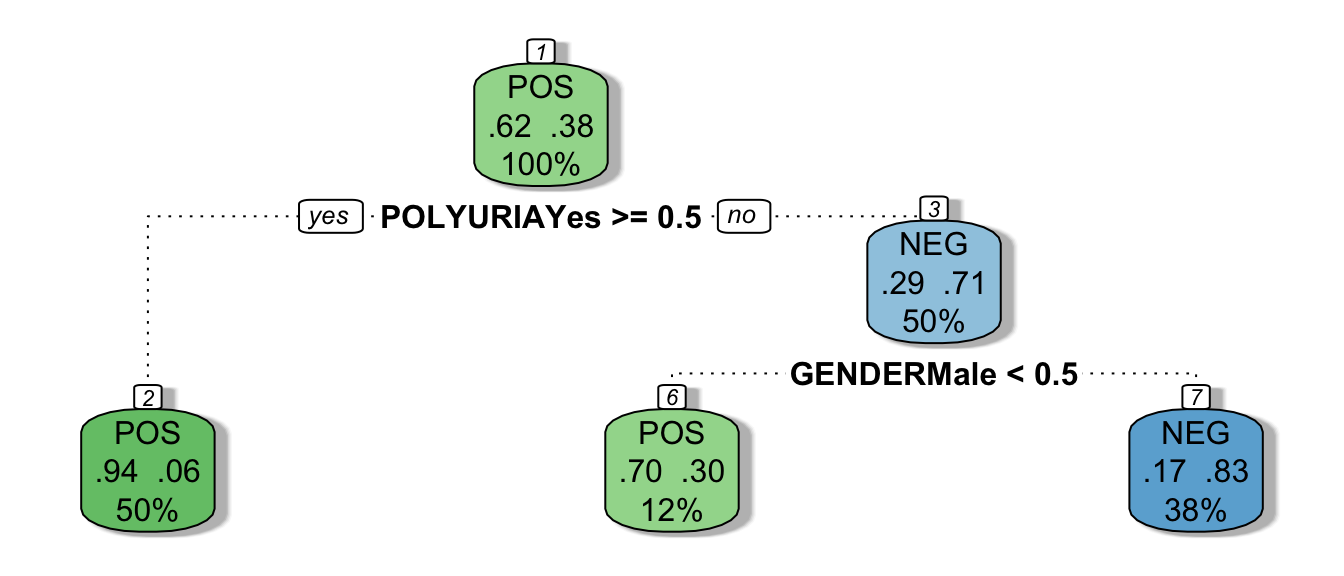
Trees created with the caret package cannot be plotted with the rpart.plot() function. Use rattle::fancyRpartPlot() instead.
Loading required package: bitopsRattle: A free graphical interface for data science with R.
Version 5.4.0 Copyright (c) 2006-2020 Togaware Pty Ltd.
Type 'rattle()' to shake, rattle, and roll your data.
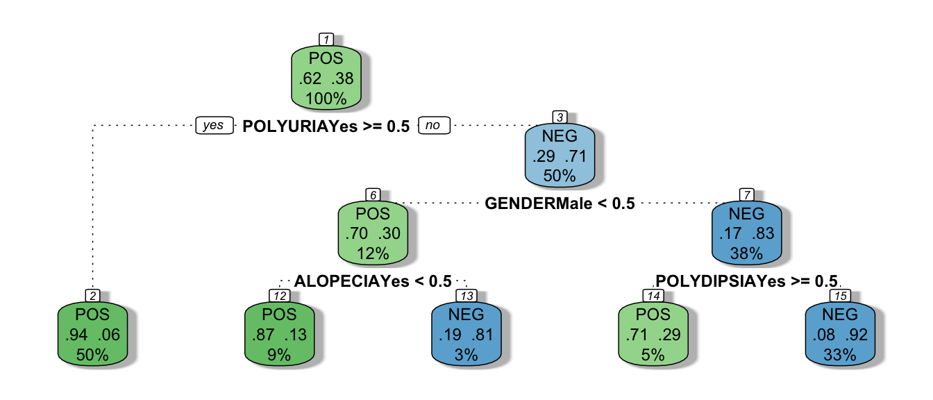
The tree created with the defaults of caret is a pruned version of the tree created with the default settings of rpart. It is possible to create a less pruned tree in caret by tuning the hyper parameters. Rpart also offers options to tune the training process.
In general, it is good practice to start with the default settings and, after some experience, go deeper into model tuning.
5.2.0.4 Model tuning in caret
The strength of the caret package lies in the diversity of ML models that are built into this package and the possibilities to tune the model. To learn and understand the concepts behind an ML model, it is better to use a package developed for the specific ML model. E.g. use rpart (or tree) to better understand the concepts of buidling a decison tree model.
The model in the previous example in caret was built using bootstrapping. It is easy to use another technique instead, e.g. (repeated) Cross Validation. The output showed the cp parameter which was used to tune the model, by default caret tested three different cp values. Testing more cp values is a matter of using extra arguments in the train() function.
See the example below in which Cross Validation is used instead of Bootsttrapping and in which more values for cp are tested.
library(rattle)
trctrl <- trainControl(method = "cv", #cross validation
                       number = 10)   #10-fold cross validation
cp_grid <- data.frame(cp = seq(0.02, .2, .02))

tree_03 <- train(CLASS~., data = df_prep, method = 'rpart',
                 trControl = trctrl,
                 tuneGrid = cp_grid)

tree_03
CART
520 samples
16 predictor
2 classes: 'POS', 'NEG'
No pre-processing
Resampling: Cross-Validated (10 fold)
Summary of sample sizes: 468, 468, 468, 468, 468, 468, ...
Resampling results across tuning parameters:
cp Accuracy Kappa
0.02 0.9134615 0.8150286
0.04 0.9076923 0.8007938
0.06 0.8788462 0.7404646
0.08 0.8711538 0.7275207
0.10 0.8711538 0.7275207
0.12 0.8384615 0.6690638
0.14 0.8230769 0.6477028
0.16 0.8230769 0.6477028
0.18 0.8230769 0.6477028
0.20 0.8230769 0.6477028
Accuracy was used to select the optimal model using the largest value.
The final value used for the model was cp = 0.02.