Chapter 5 Taylor Series

One of the most useful tools for solving problems in mathematics is the capability to approximate an arbitrary function using polynomials. There are a number of different methods for approximating functions that you will find out about in your degree including - Taylor series - Fourier series - Interpolation - wavelets (maybe) - radial basis functions (Jeremy’s research area) - neural networks (Alexander Gorban’s and Ivan Tyukin’s research areas).

5.1 Taylor polynomials

We use polynomials because they can be computed on a machine only using multiplication and addition.

Definition 5.1 A polynomial is a function of the form $$p_n(x) = \sum_{i=0}^n a_i x^i,$$ for some $n \in {\mathbb N}$. We call this a monomial, if there is only one term in this expansion. The number $n$ is called the degree of the polynomial (we assume that $a_n \neq 0$).

We have already met one Taylor polynomial, in Section 3.1 when we were looking at approximating a function by its tangent in Newton’s method. The idea for Taylor series is that we will match the each derivative of a polynomial with the derivative of the function at a particular point $b$ (this is called Hermite interpolation’’ in the trade).

We are going to start with the simple case $b=0$. Let us try with a degree 2 polynomial and an arbitrary function $f$. Let $$p_2(x) = a_0+a_1 x +a_2 x^2, \tag{5.1}$$ and we want $$\begin{eqnarray} p_2(0) & = & f(0), \\ p_2^{'}(0) & = & f^{'}(0), \\ {\rm and} \; p_2^{''}(0) & = & f^{''}(0). \\ \end{eqnarray}$$ If we let $x=0$ in (5.1) we get $$a_0 = f(0).$$ Let us now differentiate $p_2^{'}(x)=a_1+2a_2 x$. If we substitute $x=0$ we get $$p_2^{'}(0)=a_1=f^{'}(0).$$ Differentiating a second time we get $p_2^{''}(x)=2a_2$. Substituting in $x=0$ gives $$p_2^{''}(0)=2a_2=f^{''}(0),$$ so that $$a_2 = {f^{''}(0) \over 2}.$$ Therefore our approximating polynomial is $$p_2(x)=f(0)+f^{'}(0) x+{f^{''}(0) \over 2}x^2. \tag{5.2}$$

Example 5.1 Let us test the idea out on a particular function $f(x)=\sqrt{1+x}$. Then $$\begin{eqnarray} f(0) & = & \sqrt{1} = 1 \\ f'(x) & = & {1 \over 2 \sqrt{1+x}} \Rightarrow f'(0)={1 \over 2} \\ f''(x) & = & -{3 \over 4 (\sqrt{1+x})^3} \Rightarrow f''(0) = {3 \over 4}. \end{eqnarray}$$ Substituting into (5.2) we get $$P_2(x)=1+{x \over 2} - {3x^2 \over 8}x^2.$$

Now let us see if this is a good approximation. Let us use the last equation to approximate $\sqrt{1.1}=1.0488088$ to 7 decimal places. Our approximation is $$P_2(0.1) = 1+{0.1 \over 2} - {3 (0.1)^2 \over 8} = 1.04625.$$ Hence our estimate is out by approximately $0.003$.

Suppose we approximate $\sqrt{1.2}=1.0954451$ to 7 decimal places. Our approximation is $$P_2(0.2) = 1+{0.2 \over 2} - {3 (0.2)^2 \over 8} = 1.085.$$ Hence our estimate is out by approximately $0.01$, so the error has increased significantly. We will return to theoretical error estimates for Taylor series next semester.

We can see above that the higher the degree of the polynomial approximation, the better it gets. In this link

(http://mathfaculty.fullerton.edu/mathews/a2001/Animations/Interpolation/Series/Series.html)

you can examples of Taylor series approximations for a variety of functions and observe how they improve as you increase the degree of the polynomial.

More generally, we can look at the Taylor series for a point $b$. In order to compute this it is more convenient to use a different basis for the polynomials. A basis is an idea that you will see more of in linear algebra. It is a set of objects which we use to represent our information. For the point $b$ I would like my polynomial to be written in the form $$p_n(x)=a_0+a_1(x-b)+a_2(x-b)^2+\cdots+a_n(x-b)^n = \sum_{i=0}^n a_i(x-b)^i.$$ It will become clear in a second why this is a good idea. We will find $a_i$ by matching the $i$th derivative of $p_n$ with the $i$th derivative of our target function $f$, which we are trying to approximate. If we differentiate $p_n$ $j$ times we get $$p_n^{(j)}(x) = j! a_j+(j+1)!a_{j+1}(x-b)+{(j+2)! \over 2}(x-b)^2+\cdots+a_n{n! \over (n-j)!}(x-b)^{n-j}.$$ If we put $x=b$ in this we see that $$p_n^{(j)}(b) = j! a_j.$$ Since we wish to make $p_n^{(j)}(b)=f^{(j)}(b)$, we obtain $$a_j = {f^{(j)}(b) \over j!}.$$ If we had used $$p_n (x)=a_0+a_1x+a_2x^2+\cdots+a_nx^n,$$ then all of the terms greater than the $j$th term would not have become 0 and we would have got a horrible mess. Thus we have the following definition for the Taylor polynomial:

Definition 5.2 (Taylor polynomial) Let $f$ have $n$ continuous derivatives at $b$. Then the Taylor polynomial for $f$ at $b$ is $$\sum_{j=0}^n {f^{(j)}(b) \over j!} (x-b)^j$$

Definition 5.3 (Taylor series) Let $f$ have infinite continuous derivatives at $b$. Then the Taylor series for $f$ at $b$ is $$\sum_{j=0}^\infty {f^{(j)}(b) \over i!} (x-b)^j$$

Remark. The selection of a good basis is one of the most important mathematical skills to develop. A bad choice of basis can make the problem almost impossible to solve. A good choice can make it trivial.

Example 5.2 The Taylor series for $\cos x$ and $\sin x$ at $b=0$ are $$\cos x = \sum_{j=0}^\infty {(-1)^j \over (2j)!} x^{2j},$$ $$\sin x = \sum_{j=0}^\infty {(-1)^{2j+1} \over (2j+1)!} x^{2j+1}.$$

5.2 Polar form for complex numbers

Richard Feynman, the famous physicist called the following equation our jewel'' andthe most remarkable formula in mathematics’’.

Richard Feynmann

Theorem 5.1 (Polar coordinates for complex numbers) For any real number $\theta$ $$\exp(i \theta) = \cos \theta + i \sin \theta.$$

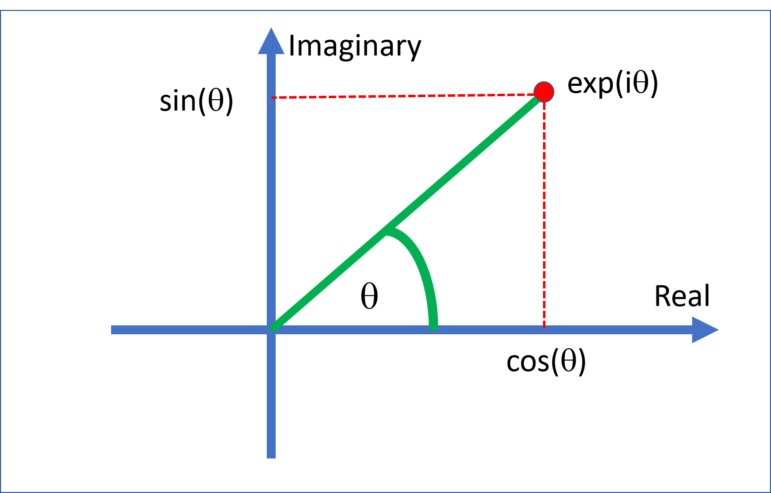
Using the Taylor series for $\exp(i \theta)$ we have $$\begin{eqnarray*} \exp(i \theta) & = & \sum_{n=0}^\infty {(i \theta)^n \over n!}\\ & = & \sum_{n=0}^\infty {i^n \theta^n \over n!}. \end{eqnarray*}$$ Now, $i^2=-1$, $i^3=-i$ and $i^4=1$, so that $$\begin{eqnarray*} \exp(i \theta) & = & \sum_{n=0}^\infty {i^n \theta^n \over n!} \\ & = & 1+i \theta - {\theta^2 \over 2!} - i{\theta^3 \over 3!}+{\theta^4 \over 4!}+{\theta^5 \over 5!}- \cdots \\ & = & 1 - {\theta^2 \over 2!}+{\theta^4 \over 4!}+ \cdots + i (\theta - {\theta^3 \over 3!} + {\theta^5 \over 5!} + \cdots) \\ & = & \left (\sum_{n=0}^\infty {(-1)^n \over (2n)!} \theta^{2n} \right )+i\left ( \sum_{n=0}^\infty {(-1)^{2n+1} \over (2n+1)!} \theta^{2n+1} \right ) \\ & = & \cos \theta + i \sin \theta. \end{eqnarray*}$$

Thus $\exp(i \theta)$ is a complex number with real part $\cos \theta$ and imaginary part $\sin \theta$. If plot this we can see that $\exp(\theta \theta)$ is a complex number of length 1 at angle $\theta$ to the real axis.

Polar coordinates

Definition 5.4 (Polar form of complex number) Any complex number can be written in polar form $$z=x+iy=r\exp(i \theta),$$ where $r=\sqrt{x^2+y^2}$ is called the of the complex number (written $|z|$, and $\theta=\arctan(y/x)$ is called the argument of the z, written ${\rm arg \,} z$.

Example 5.3 Write $z=2+4i$ in the form $z=r\exp(i \theta)$.

The modulus of $z$ $r=\sqrt{2^2+4^2}=\sqrt{20}$. We have $\theta={\rm arg \,} z=\arctan(4/2)=1.11$ radians.