Chapter 3 Differentiation

In this chapter we will introduce the idea of differentiation. Of course, you have been able to differentiate for a couple of years now, so we will not focus on the mechanics of differentiation, but rather on the ideas behind it, so that you can use these ideas flexibly in any problem you may be required to solve. At the following link you can find out more about the history of the derivative:

http://www.math.wpi.edu/IQP/BVCalcHist/calc2.html

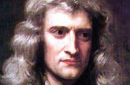
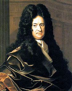
The two scientists that are credited with the main formalism around differentiation are Newton and Leibnitz. Their pictures are below, Newton and the Leibnitz:

Interestingly there are biscuits named after these two mathematicians - here they are, the fig newton and the chocolate Leibnitz:

The main reason we want to differentiate is to find the rate of change of something. If that something is the rate of change of height with distance, then we are finding the gradient. This is useful for understanding how steep roads are for instance. If we want to find out the rate at which distance changes with time then we are computing the speed of something.

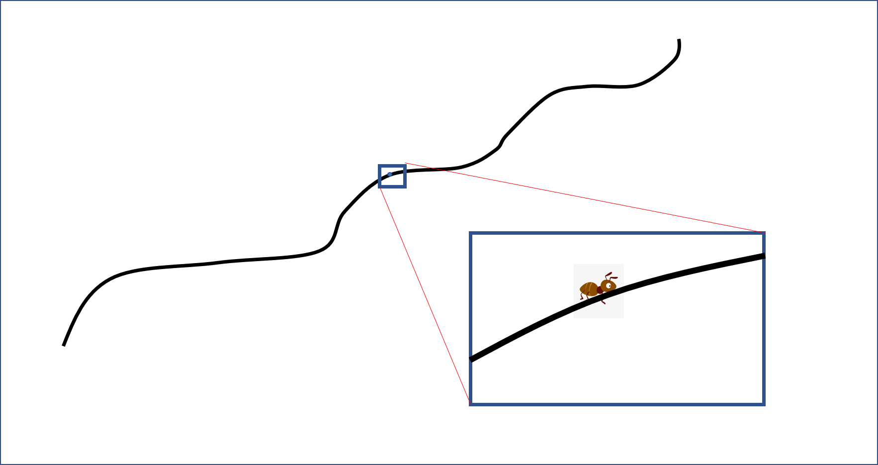
Here is a video about differentiation that you might find interesting:

The main idea is that if I am very small then all slopes look like straight lines. To the ant all roads look flat. In order to make the slope look flat I just have to look close enough. This is the idea of the limit. For a straight line we know how to calculate the gradient:

ant

Key idea: the derivative is calculated by considering such a small change in the independent variable \(x\) that the dependent variable \(y\) depends linearly on \(x\) in that time interval. Another way of thinking about this is to say that the function is represented by its tangent (is a straight line). More formally we define this as a limit.

Definition 3.1 The derivative of the function \(f(x)\) at a point \(a\) is the rate of change of \(f\) at \(a\), or the slope of the tangent to the curve. It is denoted by \[ {d f \over dx} \; {\rm or} \; f'(x). \] This can be computed using the idea of limit \[ {d f \over dx} = \lim_{h \rightarrow 0} {f(x+h)-f(x) \over h}. \] The value of \(h\) controls the magnification that you need in order for the function to be locally a straight line.

Example 3.1 Find the derivative of \(f(x)=x^2\) at the point \(x=2\). To do this we compute \[ \lim_{h \rightarrow 0} {f(2+h)-f(2) \over h} = \lim_{h \rightarrow 0}{(2+h)^2-2^2 \over h} = \lim_{h \rightarrow 0}{4+4h+h^2-4 \over h} = \lim_{h \rightarrow 0} (4+h) = 4. \]

In the next bit of code you can compute the derivative of any function at any point using this definition.

3.1 Newton’s method for solving non-linear equations

Solution of non-linear equations is one of the most important applications of mathematics. These are used to optimise complicated processes.

Example 3.2 We want to construct a box whose base length is 3 times the base width. The material used to build the top and bottom cost \(10\) pounds per square metre and the material used to build the sides cost \(6\) pounds per square metre. If the box must have a volume of \(5 {\rm m}^3\) determine the dimensions that will minimize the cost to build the box.

The box is made up of a base and a lid, plus four sides. Two of the sides are length times height and two are width times height. If \(w\) is the width, \(l\) is the length and \(h\) is the height, we have \(l=3w\). The volume is \(lwh=5\), so that \(h=5/(lw)=5/(3w^2)\). Hence the cost of the box \[ C(w)=2lw \times 10 + 2lh \times 6 + 2 wh \times 6 = 60w^2+{80 \over w}. \] To find when this is a minimum we must differentiate and solve \[ C'(w)=120w-{80 \over w^2}=0. \]

We will get back to solving this later.

Newton’s method finds the root of a nonlinear equation (like \(x^2-2=0\)) by pretending that the function is a straight line (if we are ant it is true), and finding the root of the linear equation. This gives a better guess than before. Then we repeat this, in other words, iterate.

The following image is from (https://www.math24.net/newtons-method/) and you can get a number of examples there to practice. In the image you can see the first guess \(x_0\). Then we construct the (green) tangent at \((x_0,f(x_0))\). The interesection of this line with the \(x\)-axis is \(x_1\). We then construct the (red) tangent at \((x_1,f(x_1))\). The intersection of this line with the \(x\)-axis is \(x_2\). Rinse and repeat. YOu can see we get closer and closer to the intersection of the function with the \(x\)-axis.

Here is a webpage where you can see this iteration process happening, and try to solve your own equations.

(https://www.intmath.com/applications-differentiation/newtons-method-interactive.php)

In order to implement the idea we need to work out the equation of the tangent line to a curve at a point.

Theorem 3.1 The equation of the tangent to a function \(y=f(x)\) at a point \(a\) is \[ y=f(a)+(x-a)f'(a). \]

**Proof:} The equation of a straight line through a point is, in general, \(y=mx+c\). Now, the gradient of the line at \(a\) is the derivative of the function at \(a\): \(f'(a)\). Thus the equation of the line is \[ y=xf'(a)+c. \] We choose \(m\) so that the line goes through the point \((a,f(a))\). Hence \[ f(a)=af'(a)+c \] so that \(c=f(a)-af'(a)\). Hence \[ y=xf'(a)+f(a)-af'(a)=f(a)+(x-a)f'(a). \quad \Box \]

For Newton’s method we find where the tangent cuts the \(x\)-axis and use this as a next guess. Hence we solve \[ y=f(a)+(x-a)f'(a)=0, \] so that \[ x=a-{f(a) \over f'(a)}. \]

Thus we have the equation for Newton’s iteration \[ x_{n+1}=x_n-{f(x_n) \over f'(x_n)}. \tag{3.1} \]

Here are some animations demonstrating Newton’s method

(http://mathfaculty.fullerton.edu/mathews/a2001/Animations/RootFinding/NewtonMethod/NewtonMethod.html)

Example 3.3 Find the cube root of 9.

To do this we need to solve the equation \(x^3-9=0\). We will use Newton’s iteration . We have \[ f'(x)=3x^2. \] Hence the iteration is \[ x_{n+1}=x_n-{x_n^3-9 \over 3x_n^2}. \] Let us start with \(x_0=2\) because we know that this is the cube root of 8, which is not far away. Then \[\begin{eqnarray*} x_1 & = & x_0-{x_0^3-9 \over 3x_0^2} = 2-{-1 \over 12} = 2.080088888888889.\\ x_2 & = & x_1-{x_1^3-9 \over 3x_1^2} = 2.080083823064241.\\ x_3 & = & x_2-{x_2^3-9 \over 3x_2^2} = 2.080083823051904.\\ x_4 & = & x_3-{x_3^3-9 \over 3x_3^2} = 2.080083823051904. \end{eqnarray*}\]

Here is some R code which does the heavy lifting for you in this iteration. Of course you can change the code to solve any equation you like.

fun = function(x){
  x^3-9
}

dfun=function(x){
  3*x^2
}

options(digits=12) # Print answers to 12 digits

epsilon <- 10^{-10} # Terminate the iteration when the difference is less than epsilon

xold <- 2 # Starting point

xnew <- xold-fun(xold)/dfun(xold) # first Newton iteration

print(xnew) # write the answer to the screen

## [1] 2.08333333333

while (abs(xnew-xold) > epsilon){
  
  xold <- xnew # use the new point for the next iteration
  
  xnew<-xold-fun(xold)/dfun(xold) # Newton iteration
  
  print(xnew) # write the answer to the screen with 12 decimal places
}

## [1] 2.08008888889
## [1] 2.08008382306
## [1] 2.08008382305

cat("Solution is", xnew) # print answer with a comment in front of it

## Solution is 2.08008382305

Remark. The sequence above is another example of a Cauchy sequence as the distance between consecutive numbers in the sequence is getting smaller and smaller. How much smaller are the errors getting? One of the questions we will return to is how to prove what we observe here.

Example 3.4 Adapt the code above to solve the equation from Example 3.2.

3.2 Properties of the derivative

You are all accustomed to all of the standard properties of the derivative, so we are not going to prove any of these here. You did them in A level. Here is a webpage with all of the appropriate properties.

Here are the properties you need for the moment.

Theorem 3.2 (Properties of differentiation) Let \(f\) and \(g\) be differentiable functions. Then if \(\alpha, \beta \in {\mathbb R}\), \(\alpha f+\beta g\) and \(fg\), are differentiable, and \(f/g\) is at all points \(x\) with \(g'(x) \neq 0\). Furthermore,

• \((\alpha f+\beta g)'=\alpha f'+ \beta g'\);
• \((fg)'=f'g+fg'\);
• \((f/g)' = (f'g-fg')/g^2\) at all points \(x\) where \(g'(x) \neq 0\).

3.3 The fundamental theorem of calculus

The reason that you were shown integration from first principles first is that it is a process independent of differentiation. It is often taught as antidifferentiation, but the fact that this is true is one of the great theorems of mathematics. This explains the conundrum presented to you in your induction pack

Why is the derivative of the area of a circle its circumference?

We are going to use the idea of integral as the area under a curve. So suppose \[ F(x) = \int_a^x f(t) dt. \]

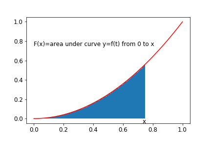
Fundamental theorem of calculus 1

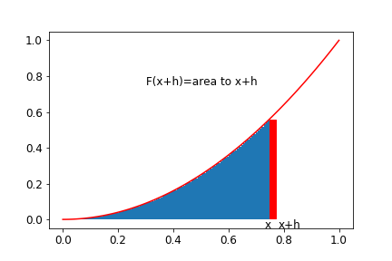
Then \[ F(x+h) = \int_a^x f(t) dt; \] see the figure below.

Fundamental theorem of calculus 2

The difference in the areas is the red rectangle which has height \(f(x)\) and width \(h\). Hence \[ F(x+h)-F(x) \approx h f(x), \] so that \[ {F(x+h)-F(x) \over h} \approx f(x). \] As \(h\), the width of the red rectangle , gets smaller the rectangle gets to be a better and better approximation to the actual area under the curve. Thus \[ lim_{h \rightarrow 0} {F(x+h)-F(x) \over h} \approx f(x). \]

Theorem 3.3 (The fundamental theorem of calculus) Let \(a \in {\mathbb R}\) and \(x>a\). Let \[ F(x)= \int_a^x f(t) dt. \] Then \(F'(x)=f(x)\).

This is not a formal proof, but gives the idea of the proof. If you do not understand the idea, then you will never be able to understand the formal proof. Mathematical analysis is the tool by which we justify all the arm waving arguments I made above. We call this being rigorous.