Chapter 2 Why Differential Equations?

2.1 Rates of Change

Many problems are difficult to solve. Many relationships that we want to understand, i.e. functions, are not readily available. For these situations, we need to develop tools – mathematical tools. Consider the altitude of a fighter aircraft. We do not necessarily have a function that simply gives us altitude at any prescribed time. Instead, we have known forces produced by jet engines impacting a known airframe. Using Newton’s Second Law of Motion $\left( F = ma \right)$, we can convert a known force into a vertical acceleration, but acceleration is not altitude. We need a means of determining altitude from vertical acceleration.

Acceleration is defined as the rate of change of velocity, $v^{'}\left( t \right) = a\left( t \right)$. Moreover, velocity is the rate of change of position which is height (altitude) in our case, $h^{'}\left( t \right) = v(t)$. There are many relationships defined by rates of change, and as we learned earlier, derivatives are rates of change! We can often find functions if we know their associated derivatives, just as we did when using integration. In the example with the fighter, we know the vertical acceleration provided by the engines and airframe, and we look to convert that rate of change knowledge into its underlying functions, namely velocity and altitude. Differential equations provide a mechanism to address these types of problems.

2.2 SIR Model

The basic SIR model is used to study the spread of disease. We consider three unknown functions; $S(t)$, the number of people susceptible to infection, $I(t)$, the number of infected and still contagious people, and $R(t)$, the number of people recovered from the disease (people who are no longer susceptible nor contagious). As we saw during the COVID pandemic, it is important to know the function for the number of infected people, $I\left( t \right)$. This function determines the need for treatments, hospitalizations, and overall patient care. Unfortunately, we do not know the function $I\left( t \right)$. However, we have a means of using differential equations to approximate it. Toward this end, we let $N$ be the total population under consideration, and the SIR model is:

$$\begin{equation*} \begin{aligned} s' &= - \beta si,\\ i' &= \beta si - \gamma i,\\ r' &= \gamma i. \end{aligned} \end{equation*}$$ In this model,

• $s(t)$ is the fraction of susceptible people, i.e. $s(t) = S(t)/N$,
• $i(t)$ is the fraction of infected and contagious people, i.e. $i(t) = I(t)/N$,
• $r(t)$ is the fraction of people recovered from the disease, i.e. $r(t) = R(t)/N$,
• $\beta$ is the infection rate measured as probabilistic contacts per day,
• $\gamma$ is the recovery rate measured as a daily fraction of those infected,
• and $t$ is the independent variable time measured in days.

We start by examining the model. The rate of change for susceptible people, $s^{'}(t)$, is determined by the interactions between infected and susceptible people. As these groups interact, some of the susceptible people will become infected, so the number of susceptible people is always decreasing. This interaction is modeled using multiplication, $- \beta s(t)i(t)$. Similarly, the population of people recovered from the disease is always increasing. The rate of change for recovered people is positive and directly related to the number of people who are infected, $\gamma i(t)$. Connecting the susceptible and recovered groups are those who are actively infected and contagious. The rate of change has a positive component reflecting the susceptible people becoming infected and negative component reflecting those who are infected transitioning to no longer being contagious. Thus, the number of infected people is changing in both positive and negative directions simultaneously, $\beta s(t)i(t) - \gamma i(t)$. Because we understand these rates of change, we can build an accurate, albeit simple, model.

Next, we take a deeper look at the parameters $\beta$ and $\gamma$. Each susceptible person has $\beta i$ probability of being infected through contact where $i$ is the fraction of the population who are infected, and $\beta$ is a combination of the number of contacts per day and the probability of becoming infected during each contact. Infected people are no longer contagious after $1/\gamma$ days, on average.

We first apply the SIR model by considering a typical year with influenza. A person with the flu is generally contagious for about 3 days which gives $\gamma = \frac{1}{3}$ . The value for $\beta$ is based on empirical evidence of social interactions and the contagiousness of the flu. The resulting parameter range is: $\frac{7}{16} \leq \beta \leq \frac{1}{2}$ . We apply these parameters to our model. After applying the values of $\gamma$ and $\beta$, we are still unable to solve for $i\left( t \right)$ directly. There is no anlytical solution available. The fact that we cannot solve this system is not due to our shortcomings, but rather, it is just reality. There is no way currently available for finding $i\left( t \right)$ directly. Instead we apply a numerical algorithm to the system of differential equations and approximate the functions $s\left( t \right)$, $i\left( t \right)$, and $r\left( t \right)$.

The following graphs show the resulting functions that are approximated using the SIR model. The two graphs depict the endpoints of our $\beta$ interval, i.e. $\beta = \frac{1}{2}$ and $\beta = \frac{7}{16}$ .

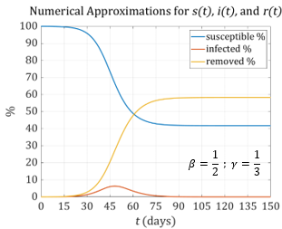
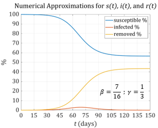
Notice the significant differences in the graphs. With $\beta = \frac{1}{2}$ the maximum number of infections is approximately 6.5% of the total population. With $\beta = \frac{7}{16}$ the maximum drops to about 3%. We can see the importance of accurately determining $\beta$ and $\gamma$.

During the COVID pandemic, the world faced a new disease with one remarkable attribute: people remained contagious for a long period of time (approximately 8 days). Using the same probabilities as we did for the flu, we can see the impact of a longer contagious period.

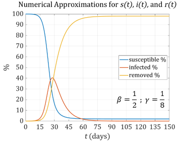
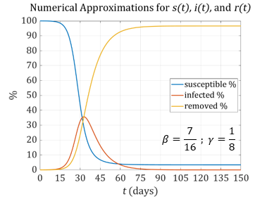
Notice that on both graphs, the fraction of the population that is infected peaks well above $35\%$. Without a reaction by the US and state governments, COVID would have spread rapidly with devastating consequences. Both models shows a peak after about 1 month with 35% - 40% of the population being infected. If only 5% of the infected people needed hospital beds, that would require enough beds for $$35\%\times 5\%\times \text{US population} = \ 0.35\times 0.05\times 330,000,000 = 5,775,000\ \text{people}.$$

The United States has approximately 1,000,000 hospital beds.

Our model is overly simplistic, but it provides a rough idea about the impact of highly contagious diseases. We are able to use a system of differential equations to understand the infection curve. As a result of this deeper understanding, the state governments in the US tried to “flatten the curve” during the COVID pandemic. They were talking about the infection curve, $i(t)$.

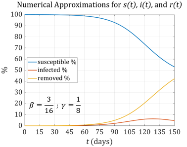
Consider driving the interactions down significantly so the associated parameter becomes $\beta = \frac{3}{16}$ . The result of this effort does flatten the infection curve, but there is one significant disadvantage of this approach. The disease persists for a much longer period of time. Again, our model is overly simplistic, but this observed longevity actually occurs as we saw with COVID. Instead of processing the disease through the country’s population in a couple of months, COVID persisted as a pandemic for a couple of years.

This type of modeling and exploration of problems, situations, and opportunities is at the heart of differential equations. Throughout this chapter, we will find solutions, interpret graphs, and approximate functions. These skills are used regularly throughout a wide variety of disciplines.