Chapter 4 Analytical Solutions for $y^{'} = f(t)$

4.1 General Solutions

We now develop a more direct way to solve some differential equations. While we can always “guess and check,” that approach is generally ineffective and is always inefficient. We start by considering a special subset of differential equations. ODEs with a right-hand side that is only a function of the independent variable, $t$, can sometimes be solved analytically. An analytical solution is one where the general solution can be found in a closed form. The Fundamental Theorem of Calculus (FToC) gives us the answer to

$$y^{'} = f(t)$$

because $y(t)$ is the antiderivative of $f(t)$.

Recall that the FToC is a critically important result that relates functions and their derivatives

$$\int_{}^{}{y^{'}(t)}dt = y(t) + C$$

To find all solutions to this type of ODE, we simply integrate both sides of the differential equation with respect to $t$. Applying indefinite integration to $y^{'} = f(t)$ yields

$$\begin{aligned} \int_{}^{}y^{'}dt &= \int_{}^{}{f(t)}dt \\ y(t) + C_{1} &= \int_{}^{}{f(t)}dt + C_{2} \\ y(t) &= \int_{}^{}{f(t)}dt + C \end{aligned}$$

Note: The constant $C_{2}$ is generated when we integrate $f(t)$. We know $C_{2}$ exists, and we can track it separately. To simplify, we combine the integration constants as $C = C_{2} - C_{1}$. We must carefully track the constants to ensure a complete and accurate solution.

4.1.1 Example #1

Solve the differential equation

$$y^{'} = e^{3t}$$

Integrating both sides of the differential equation leads to a general form for the solution

$$\begin{aligned} \int_{}^{}y^{'}dt &= \int_{}^{}e^{3t}dt \\ y(t) + C_{1} &= \frac{1}{3}e^{3t} + C_{2} \\ y(t) &= \frac{1}{3}e^{3t} + C \end{aligned}$$

We conclude by saying: $y(t) = \frac{1}{3}e^{3t} + C$ is the general solution to the ODE $y^{'} = e^{3t}$.

4.1.2 Example #2

Recall this example from the introduction

$$y^{'} = \cos(t)$$

Integrating both sides of the ODE yields

$$\begin{aligned} \int_{}^{}y^{'}dt &= \int_{}^{}{\cos(t)}dt \\ y(t) + C_{1} &= \sin(t) + C_{2} \\ y(t) &= \sin(t) + C \end{aligned}$$

Note that when we integrate both sides of an equation, we end up with a constant of integration on both sides. Next, we always combine the two constants into a single constant. Because we always do this, it is common to only include the constant of integration on one side of they ODE, typically the right side, and understand that we have already combined the constants. We follow this practice throughout the rest of the text.

4.2 Initial Value Problems

Next, we consider how a specific value for the constant $C$ can be determined. If the solution to the differential equation is known at a specific time, say $t_{0}$, then a specific solution can be identified. For example, let $t_{0} = 0$ with the value $y(0) = 1$. By applying this condition to the general solution, we can determine a unique value for $C$ as

$$\begin{aligned} &y(t) = \sin(t) + C\ \ \text{ and}\ \ \ \ y(0) = 1, \\ &y(0) = \sin(0) + C = 1, \\ &\sin(0) + C = 1. \end{aligned}$$ Because $\sin(0)=0$, we are left with $C=1$. Therefore, the solution to the differential equation, $y'(t) = \cos(t)$, with the initial condition, $y(0) = 1$, is

$$y(t) = \sin(t) + 1.$$

This solution satisfies BOTH the ordinary differential equation and the initial condition. In the figure below, all of the functions shown are solutions to the ODE. However, only the function in blue is a solution to the initial value problem. Note that the function in blue is the only solution among the family of solutions that passes through the point $(t=0,y=1)$ specified in the initial condition.

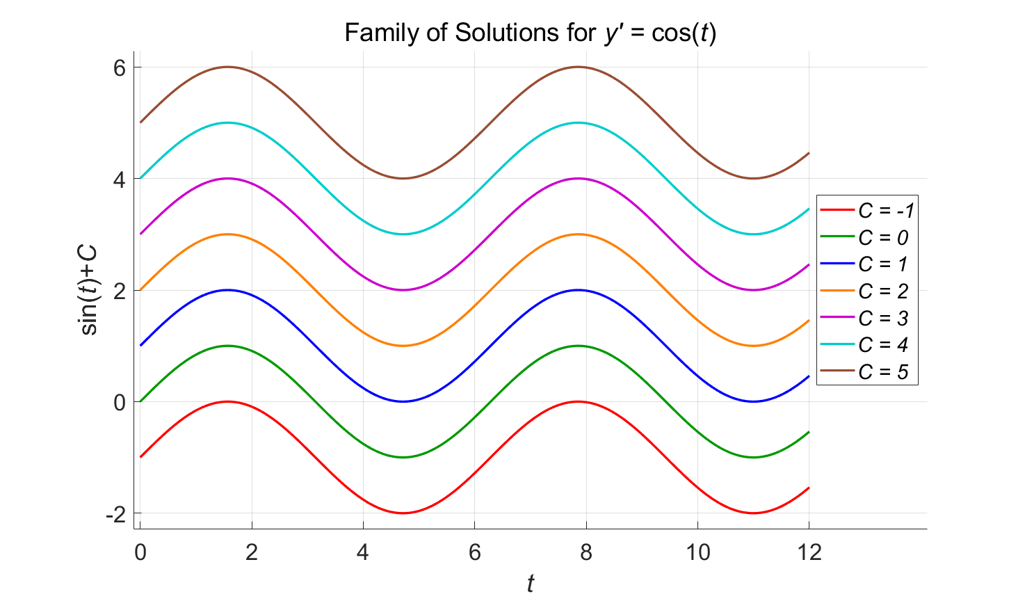
Figure 4.1: Family of Solutions for $y' = \cos(t)$. Only the function in blue satisfies the initial condition $y(0)=1$.

Some vocabulary to note:

1. An Initial Condition (IC) for an ODE is a function value, $y\left( t_{0} \right)$, provided at a specific value of the independent variable, often denoted $t_{0}$. The value, $t_{0}$, does not need to equal zero. For example: let $t_{0} = 3$, then $y(3) = 2$ would still be called an initial condition.

2. The constant of integration, $C$, is determined by applying the initial condition to the ODE’s general solution. The result is a specific solution, i.e. a solution specific to the IC.

3. When an ordinary differential equation (ODE) and initial condition (IC) are provided as a single problem, the combination is called an Initial Value Problem (IVP).

4.2.1 Example #3

Solve $$y^{'} = t\ln(t)\text{ and }y(1) = - 2, \text{assuming } t >0.$$ We begin by finding the general solution. Integrating both sides of the ODE (use integration by parts) gives

$$\begin{aligned} \int_{}^{}y^{'}dt &= \int_{}^{}{t\ln(t)}dt \\ y(t) &= \frac{t^{2}}{2}\ln(t) - \frac{t^{2}}{4} + C \\ \end{aligned}$$

Now that we have the general solution, we apply the initial condition to determine $C$. We have

$$\begin{aligned} y(1) &= - 2 = \frac{1^{2}}{2}\ln(1) - \frac{1^{2}}{4} + C \\ - 2 &= - \frac{1}{4} + C \\ C &= - \frac{7}{4} \end{aligned}$$

Substituting this value into the general solution gives us the specific solution to the IVP

$$y(t) = \frac{t^{2}}{2}\ln(t) - \frac{t^{2}}{4} - \frac{7}{4}$$

Note: this solution satisfies both the ODE and the IC. This can be easily verified.

Check the ODE:

$$\begin{aligned} &\text{LHS:}\quad y'(t) = t\ln(t) + \frac{t^{2}}{2}\left( \frac{1}{t} \right) - \frac{t}{2} = t\ln(t).\\ &\text{RHS:}\quad t\ln(t). \end{aligned}$$

Now we can check the IC by evaluating our function at $t=1$ and seeing if we get the desired value of $-2$. $$y(1) = \frac{1^{2}}{2}\ln(1) - \frac{1^{2}}{4} - \frac{7}{4} = - \frac{1}{4} - \frac{7}{4} = - 2$$

Using a direct approach and the Fundamental Theorem of Calculus is often a good method for solving IVP's when the RHS of the differential equation is only a function of the independent variable, i.e. $y^{'} = f(t)$. However, we cannot be assured of success because the function on the right-hand side may not be integrable.

For example we can try to solve this ODE

$$y^{'} = e^{- t\sqrt{t}}$$

We are stuck attempting to evaluate

$$\int_{}^{}{e^{- t\sqrt{t}}dt}$$

In these situations, we have other techniques to use. In the next few sections, we will address two approaches: Graphical Analysis and Numerical Approximation. These techniques are widely used and broadly applicable to differential equations.

The following are examples of how to solve IVPs using the Fundamental Theorem of Calculus.

4.2.2 Example #4

Find the general solution and then solve the IVP to find the specific solution:

$$u^{'} = 2t\ \text{ with} \ \ u(0) = - 2$$

Start by integrating both sides of the ODE

$$\int_{}^{}{u^{'}(t)}dt = \int_{}^{}{2t}dt$$

Applying the Fundamental Theorem of Calculus gives

$$u(t) = t^{2} + C$$

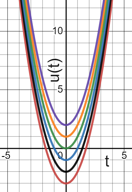
Figure 4.2: Family of Solutions for ODE in Example 4. Only one of them will solve the IVP.

The general solution is $u(t) = t^{2} + C.$

Now apply the initial condition (IC) to the general solution and find the specific solution

$$\begin{aligned} u(0) &= - 2 = 0^{2} + C \\ C &= - 2 \end{aligned}$$

The specific solution is $u(t) = t^{2} - 2$.

In the figure above we can see several solutions to the ODE. Our specific solution appears in black. Notice that the function in black passes through the point $(t=0,u=-2)$, which corresponds to the initial condition $u(0)=-2$.

4.2.3 Example #5

Find the general solution and then solve the IVP to find the specific solution:

$$z^{'} = te^{t^{2}}\ \text{ with}\ \ z(0) = 1.$$

Integrate both sides of the ODE

$$\int_{}^{}{z^{'}(t)}dt = \int_{}^{}{te^{t^{2}}}dt$$

Applying u-substitution and the Fundamental Theorem of Calculus gives

$$\begin{aligned} z(t) &= \frac{1}{2}e^{t^{2}} + C. \\ \end{aligned}$$ Below, we can see several members of the family of solutions to the ODE. Only one of them will solve the IVP.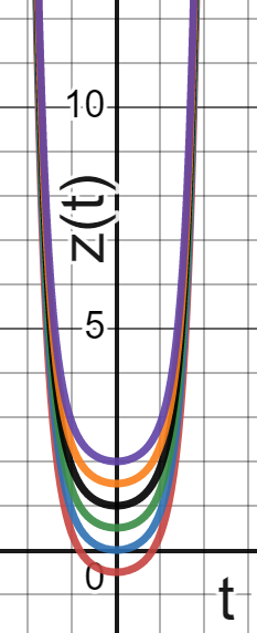

Figure 4.3: Some solutions for ODE in Example 5. Only one of these will solve the IVP.

Apply the initial condition (IC) to the general solution and find the specific solution

$$\begin{aligned} 1&=z(0) = \frac{1}{2}e^{0^{2}} + C \\ C &= \frac{1}{2}. \end{aligned}$$

The specific solution is $z(t) = \frac{1}{2}e^{t^{2}} + \frac{1}{2}$.

Again, we plot several solutions of the ODE above. Our specific solution to the IVP appears in black. Note that it passes through the point $(t=0,z=1)$, which corresponds to the initial condition $z(0)=1$.

4.2.4 Example #6

Find the general solution and then solve the IVP to find the specific solution:

$$w^{'} = t\cos(t)\ \text{ with}\ \ w(\pi) = 3.$$

Integrate both sides of the ODE

$$\int_{}^{}{w^{'}(t)}dt = \int_{}^{}{t\cos(t)\ }dt$$ Applying integration by parts and the Fundamental Theorem of Calculus gives

$$\begin{aligned} w(t) &= t\sin(t) + \cos(t) + C \\ \end{aligned}$$ Several members of the family of solutions are shown below. Only one of them will solve the IVP.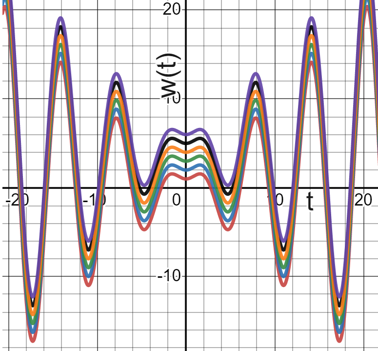

Figure 4.4: Many solutions to the ODE in Example 6. Only one of these functions will solve the IVP.

Now apply the initial condition (IC) to the general solution and find the specific solution

$$\begin{aligned} w(\pi) &= 3 = \pi\sin(\pi) + \cos(\pi) + C \\ C &= 4 \end{aligned}$$

The specific solution is $w(t) = t\sin(t) + \cos(t) + 4$.

The specific solution to the IVP appears in black in hte figure above. Note that it passes through the point $(t=\pi,w=3)$, which corresponds to the initial condition $w(\pi)=3$.

4.3 Exercises

Solve the following IVPs. Provide the general solution, the specific solution for the initial condition, and a plot of the specific solution on a representative domain. Use plotFun to plot your solutions.

#	ODE	Initial Condition
1	$y^{'} = 3$	$y(0) = - 2$
2	$u^{'} = 3t^{2} - 4t + 1$	$u(0) = - 5$
3	$w^{'} = 3\sin(t)$	$w(0) = 2$
4	$z^{'} = e^{- t}$	$z(0) = 4$
5	$w^{'} = \ln(t)$	$w(1) = 0$
6	$u^{'} = t\sin(t)$	$u(\pi) = 0$
7	$y^{'} = \frac{1}{t}$	$y(1) = 2$
8	$z^{'} = t\ e^{- t^{2}} + 1$	$z(0) = 1$
9	$y^{'} = \sin(t) + \cos(t)$	$y(0) = - 1$
10	$u^{'} = - 1$	$u(3) = 0$
11	$y^{'} = e^{t}$+1	$y(0) = - 2$
12	$u^{'} = \frac{2}{t + 1}$	$u(0) = 3$
13	$w^{'} = 3\cos(3t)$	$w(\pi) = 1$
14	$z^{'} = e^{- 3t}$	$z(0) = 2$
15	$w^{'} = \ln(5t)$	$w(1) = - 1$
16	$u^{'} = 2 - t$	$u(1) = 0$