Chapter 5 Graphical Solutions

5.1 Slope Fields and Direction Fields

Solutions to differential equations can be graphed in a variety of ways, each giving different insight into the structure of the solutions. We begin by asking what object is to be graphed. Do we first solve the differential equation and then graph the solution as was done previously? Or do we "graph" the ODE and use numerical techniques to qualitatively evaluate the solution? The first method assumes that we can find an explicit formula for the solution, i.e. an analytical solution. This is often impossible. The second method allows us to represent the ODE in a graphical manner and use numerical solvers to approximate solutions for a variety of initial conditions.

An intuitive way to graphically analyze ordinary differential equations uses slope fields. Recall the fundamental concept of ODEs relates to the equality between the rate of change, i.e. slope, of a function and the associated right-hand side expression. This construction leads directly to the idea of a slope field. Given a first order ODE

$$y^{'}(t) = f(t,y(t))$$

it is possible to compute the slope of $y(t)$, that is, $y'(t)$, if we know the current value of $y(t)$ and the current time. Using a 2D plot, these derivatives can be represented as vectors at selected points $\left( t,y(t) \right)$. The resulting plot shows the slopes at the selected points, $\left( t,y(t) \right)$, and is called a slope field. Considering each point as $\left( t,y(t) \right)$ means the horizontal axis is the $t$-axis, the vertical axis is the $y$-axis, and the vectors show the direction and magnitude of the rate of change. In particular, the vector emanating from position $(t,y)$ is a representation of the vector $(1,f(t,y))$, which has slope $f(t,y)$.

5.1.0.1 Example 1

Construct the slope field for this ODE

$$y^{'} = t^{2}\sin(t).$$

If a solution to the ODE happens to pass through the point $(t=0,y=1)$, then the ODE tells us that the slope of the solution would be $$y'(0)=0^2\sin(0)=0.$$
We represent this on the slope field by drawing a vector with slope 0 originating at the point $(t=0,y=1)$.

Similarly, if a solution happens to pass through the point $(t=1,y=1)$, we know that the derivative of the solution will be $$y'(1)=1^2\sin(1) \approx 0.84.$$ We represent this by drawing a vector with slope 0.84 emanating from the point $(t=1,y=1)$. If a solution happens to pass through the point $(t=2,y=0)$, then the solution will have slope $$y'(2)=2^2\sin(2)\approx 3.64$$ as it passes through. We represent this on the slope field by drawing a vector with slope 3.64 emanating from the point $(t=2,y=0)$

If we were to repeat this process over and over again, we would get the slope field for the ODE. The slope field is a collection of vectors that indicates the slope a solution to the ODE would have as it passed through each point. The slope field for the ODE is shown below.

We can check and see that at the point $( t=-4.2,y=1.8)$, the rate of change is given as
$$y^{'}( - 4.2) = ( - 4.2)^{2}\sin(4.2) \approx 15.375.$$

That slope is shown on the slope field by the direction and relative magnitude of the vector. The vector for this rate of change is $\begin{pmatrix} 1 \\ 15.375 \end{pmatrix}$, but a vector that large does not show up well. Thus, the software scales all the vectors to make them more presentable on the figure. Unfortunately, the auto scaling results in very small vectors closer to $t = 0$.

Often the slope vectors vary significantly in magnitude, as seen above, and the resulting slope field plot is difficult to interpret. To avoid this situation we commonly use a direction field which scales all of the direction vectors to have the same length. A direction field also shows the slope of solutions to the ODE as they pass through the base points of the vectors in the slope fields, but direction fields scale all the vectors to have the same length.

A direction field for the ODE $y'=t^2\sin(t)$ is shown below.

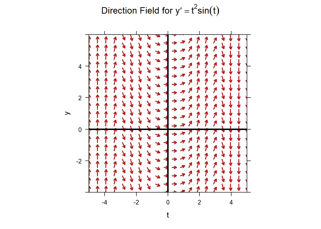
An obvious question is now: what does the direction field show us?

We know the solutions to the ODE must be tangent to the vectors. This is valuable information which allows us to approximate specific solutions, i.e. the functions $y(t)$, for different initial conditions. We will analyze the direction field for an ODE to understand the "flow" of the solutions.

Consider a vector field like a river with the various currents defined by the vectors. If we drop a volleyball into the river, then the volleyball will follow the flow defined by the vectors. The figure below shows an example of an aquamarine volleyball starting at $(t=0,y=0)$ and flowing along the ODE "river."

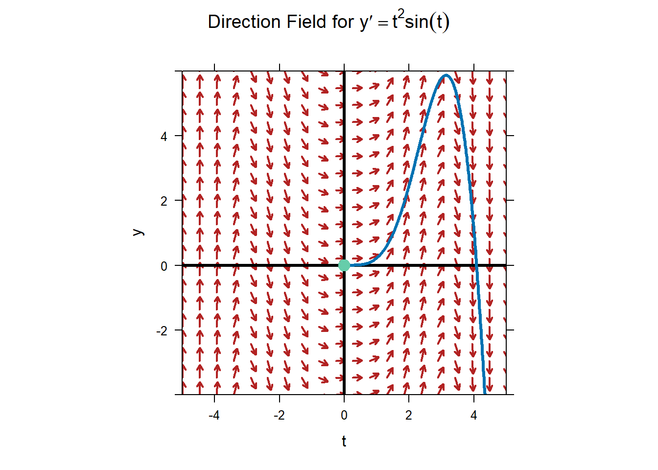
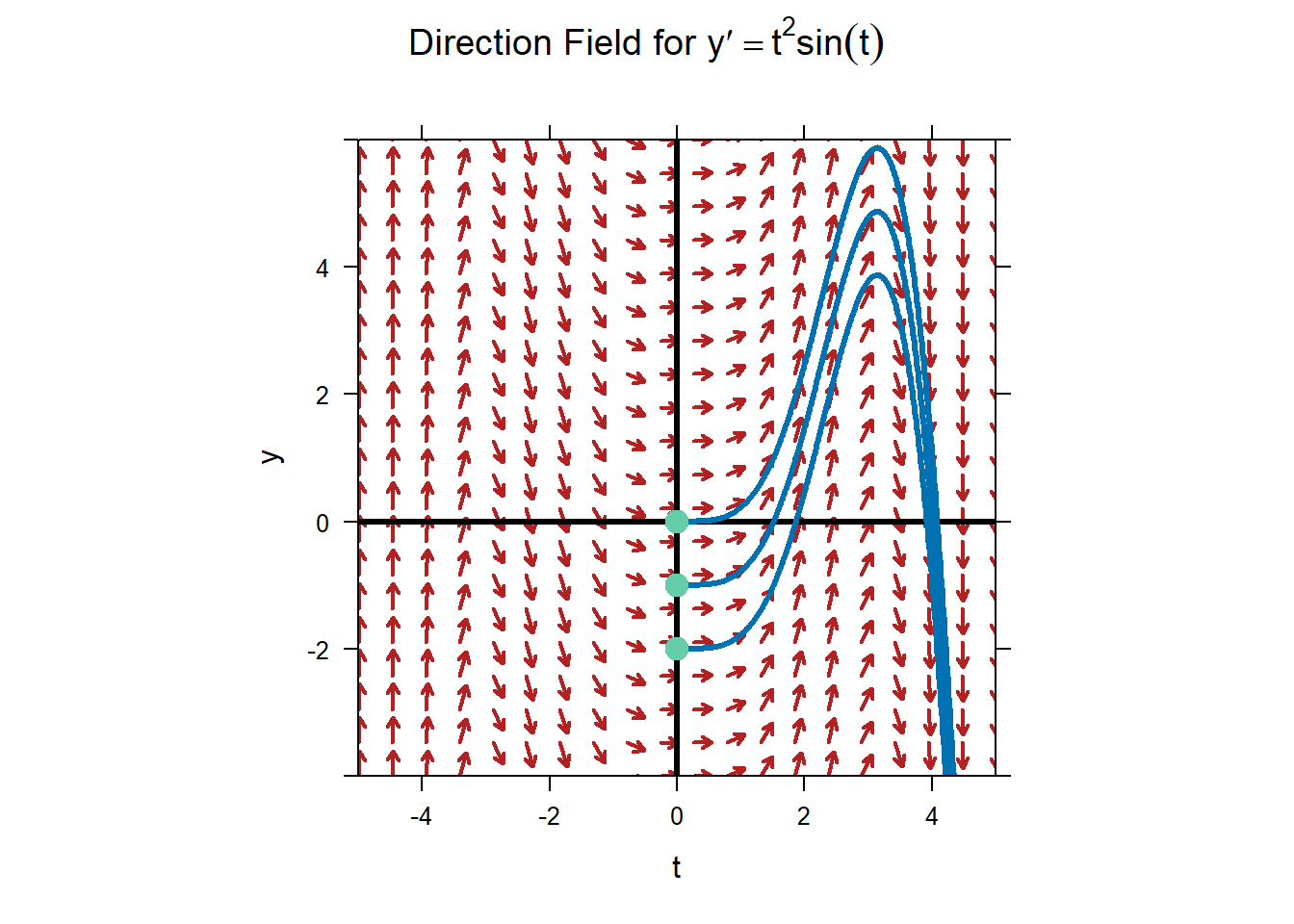
When the vector field is a direction field, our volleyball will follow the solution associated with the initial condition where the ball was dropped. We can plot multiple specific solutions simultaneously by considering multiple initial conditions. Each initial condition generates an independent solution.

The next picture shows the solutions for the ODE $$y^{'} = t^{2}\sin(t)$$ with the initial conditions: $$y(0) = 0,\, y(0) = - 1,\text{and }y(0) = - 2.$$ Notice that we also represent these initial conditions as points: $(0,0)$, $(0, - 1)$, and $(0, - 2)$, respectively.

Using direction fields, we can analyze solutions to any first order differential equation. We always know the rate of change for a 1^st order ODE, and the direction field provides us with a very useful tool.

5.1.0.2 Example 2

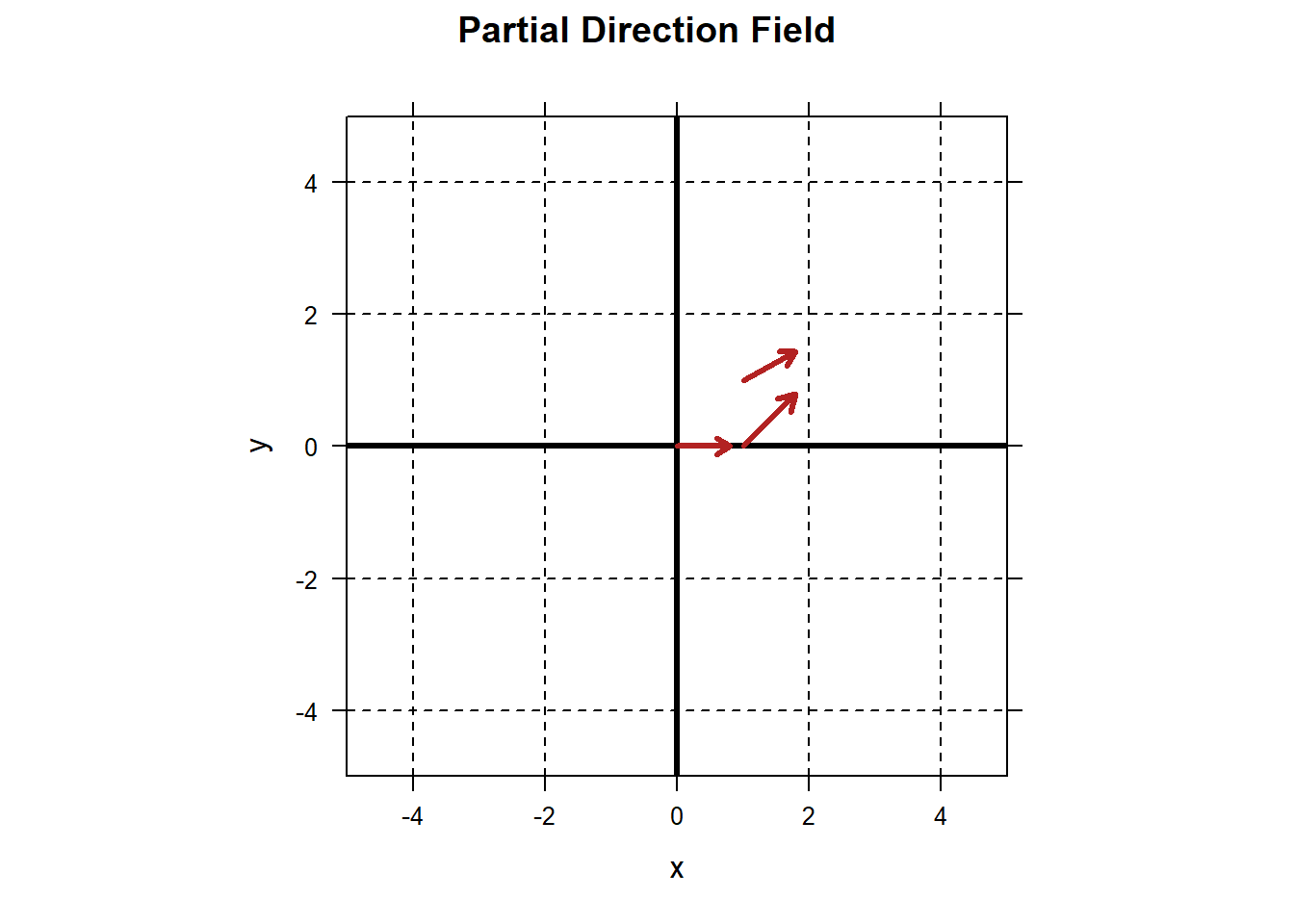
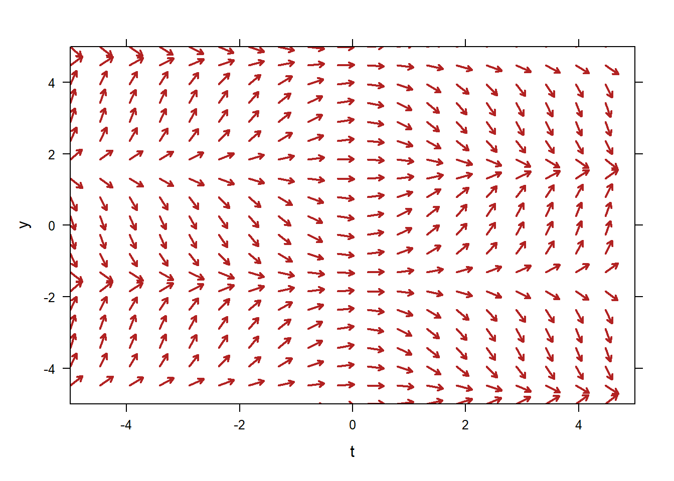
Construct the direction field for the ODE $$y'=t\cos(y).$$ Proceeding as we did before, we realize that if a solution passes through $(t=0,y=0)$, then the solution will have slope $$y'(0)=0\cdot \cos(0)=0.$$ We’ll represent that fact with a vector with slope 0 originating from the point $(0,0)$.

If a solution passes through $(t=1,y=0)$ then the solution will have slope $$y'(1)=1\cdot\cos(0)=1.$$ We’ll represent that fact with a vector with slope 1 originating from the point $(1,0)$.

If a solution passes through $(t=1,y=1)$ then the solution will have slope $$y'(1)=1\cdot\cos(1)\approx 0.54.$$ We’ll represent that fact with a vector with slope 0.54 originating from the point $(1,1)$.

Our picture at this point looks like:

This will obviously become tedious. The command plotODEDirectionField will create a direction field for you. The command below produces a complete vector field. Note that in order to tell the command that our ODE is $$y'=t\cos(y),$$ we just have to specify the right-hand side of the ODE.

plotODEDirectionField(t*cos(y)~t&y,tlim=c(-5,5),ylim=c(-5,5),col="firebrick")

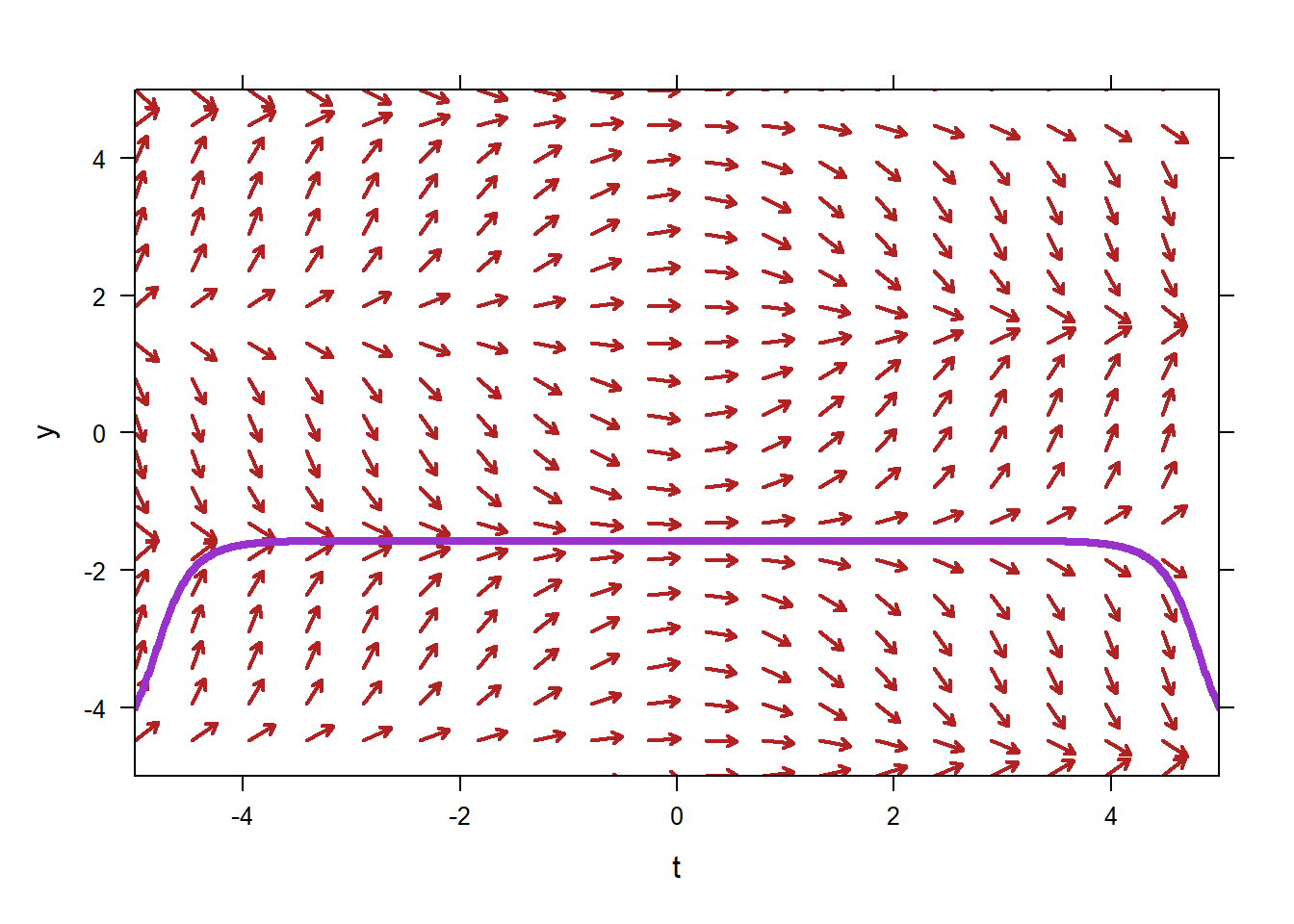
This tool can also plot specific solutions that correspond to given initial conditions. The initial condition is always assumed to be at the far-left edge of the direction field, so we need only specify the $y$-values of the initial condition. For example, to plot the solution associated with the initial condition $y(-5)=-4$, along with the direction field, we would use the following.

plotODEDirectionField(t*cos(y)~t&y,tlim=c(-5,5),ylim=c(-5,5),col="firebrick",ics=-4)

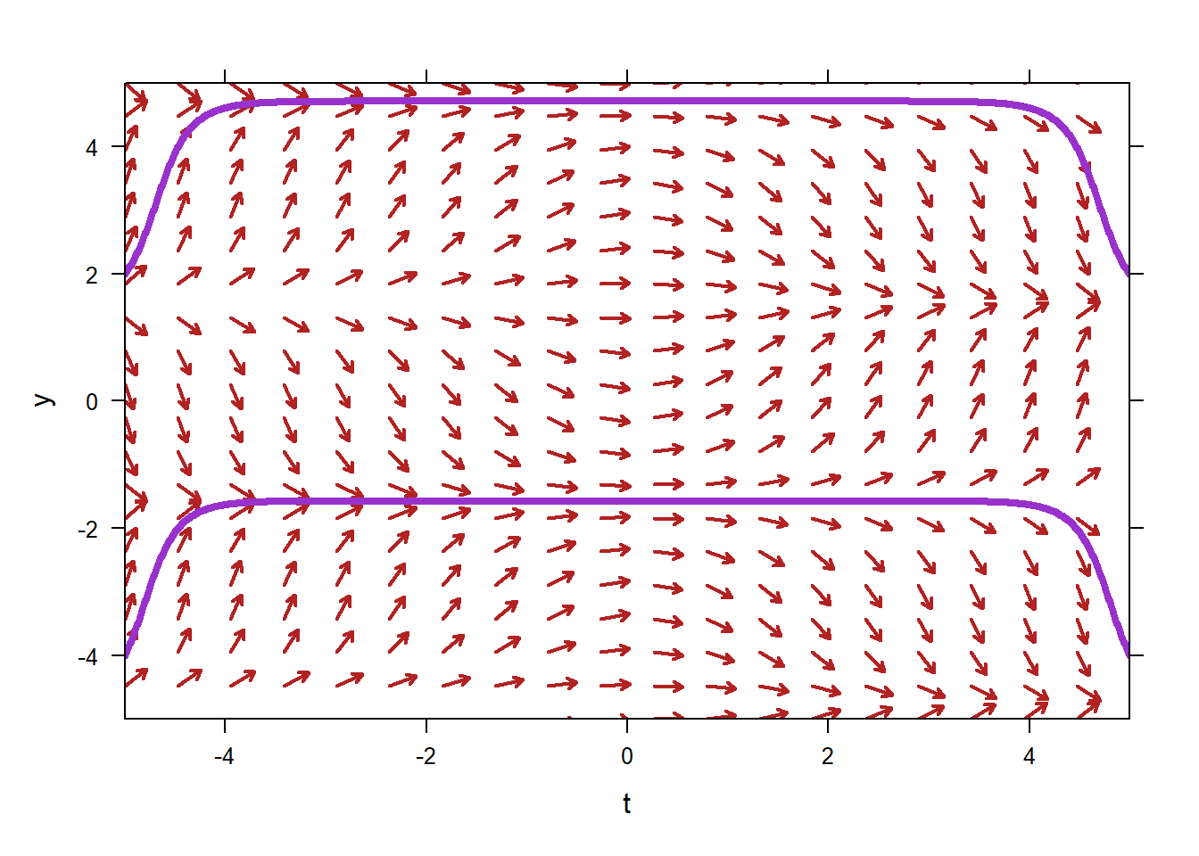
We could also specify that we want the specific solutions to the ODE with two or more initial conditions. To specify that we want the approximate solutions whose initial conditions are $y(-5)=-4$ and $y(-5)=2$ we use the command below.

plotODEDirectionField(t*cos(y)~t&y,tlim=c(-5,5),ylim=c(-5,5),col="firebrick",ics=c(-4,2))

5.2 Pure-Time and Autnomous Differential Equations

Classification of ODE is a large part of the study of ODEs. We develop specialized tools for solving ODEs based on their classifications. One important type of ODE that we have seen already are pure-time ODE. An ODE is called pure-time if it can be put in the form $$y'=f(t).$$ That is, it is pure-time if the right-hand side of the equation does not depent on $y$, only on $t$. An example of a pure-time ODE is $$y'=t\cos(t).$$ On the other hand, the ODE $$y'=t\cos(t)+y$$ is not pure-time, since $y'$ depends on both $t$ and $y$.

As we have already seen, we can frequently solve pure-time ODEs analytically by anti-differentiating.

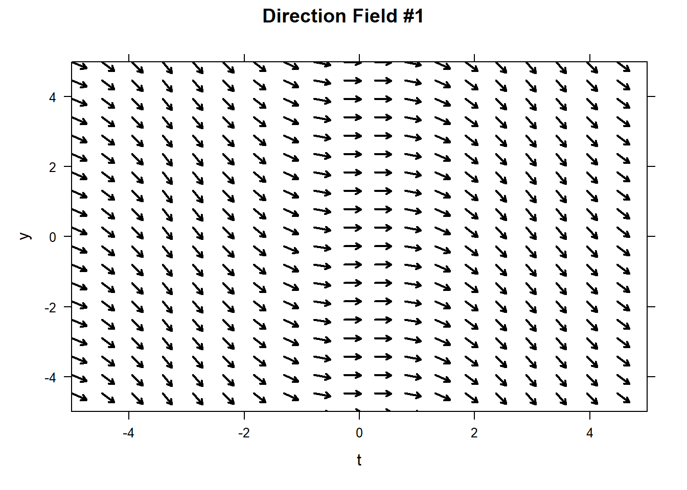
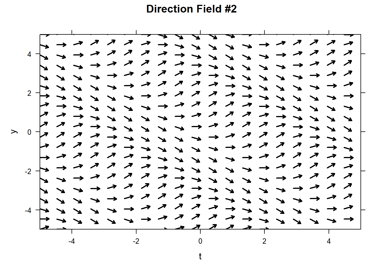
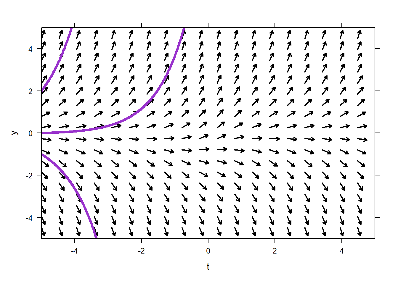
One interesting aspect of pure-time ODE is that their direction field does not vary in the $y$-direction, since by definition the slope of all solutions depend only on $t$. Below are two direction fields for two different, unspecified, ODEs. We can be sure that the ODE specified on the left is pure-time, because the vectors do not vary slope in the $y$-direction. On the other hand, the ODE represented on the right must not be pure-time.

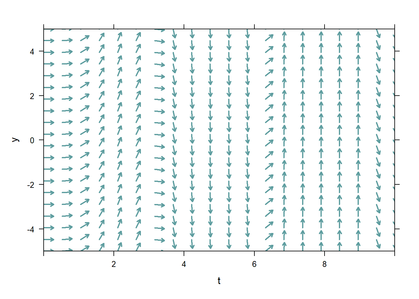
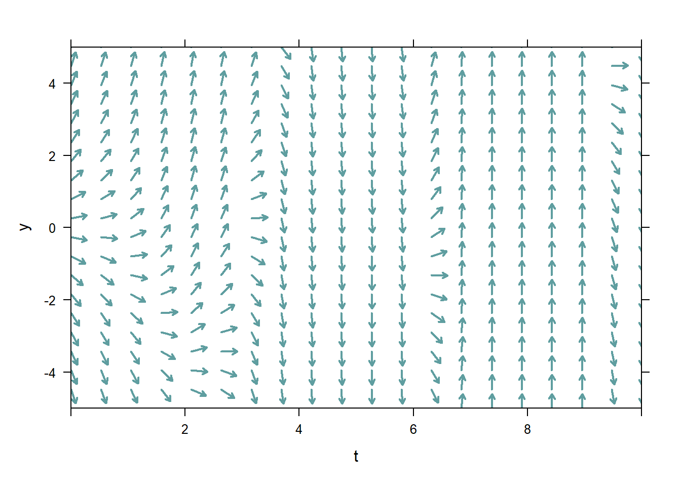
Figure 5.1: Pure-time and not pure-time ODE direction fields

The opposite of a pure-time ODE is an autonomous ODE. An ODE is autonomous if it can be put in the form $$y'=f(y).$$ That is, it is autonomous if $y'$ depends only on $y$, not on $t$.

The ODE $$y'=3y$$ is autonomous, while $$y'=3yt$$ is not.

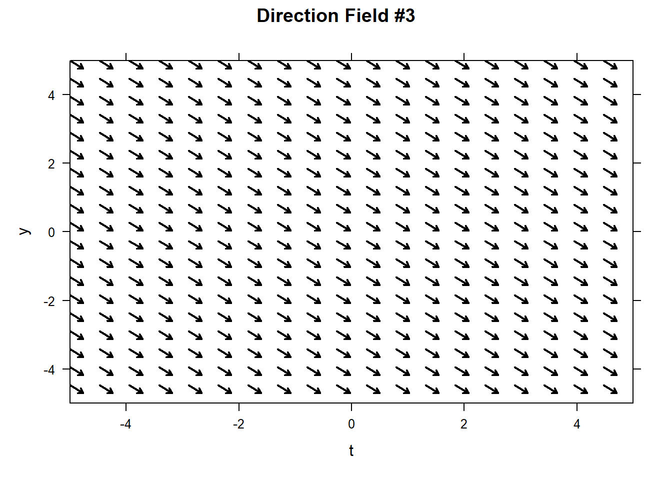
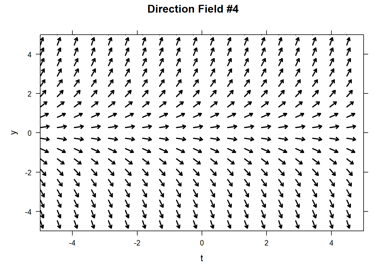
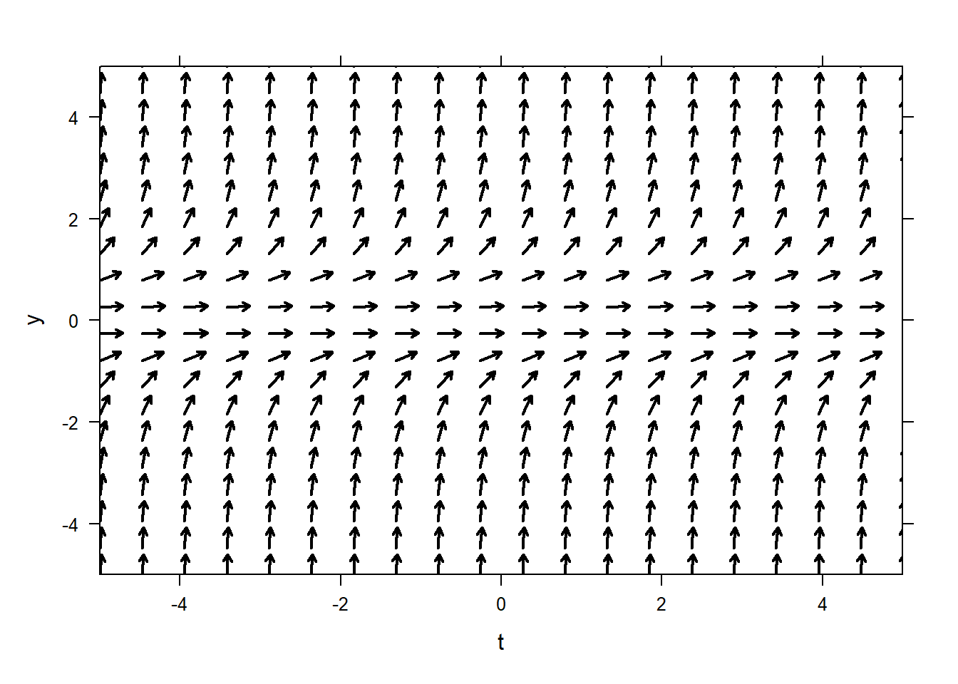
Because the value of $y'$ depends only on $y$, the slopes of the vectors in the direction field for an autonomous ODE will not vary in the $t$-direction. In the figures below, the ODE represented on the left must be autonomous, while the ODE represented on the right must not be autonomous.

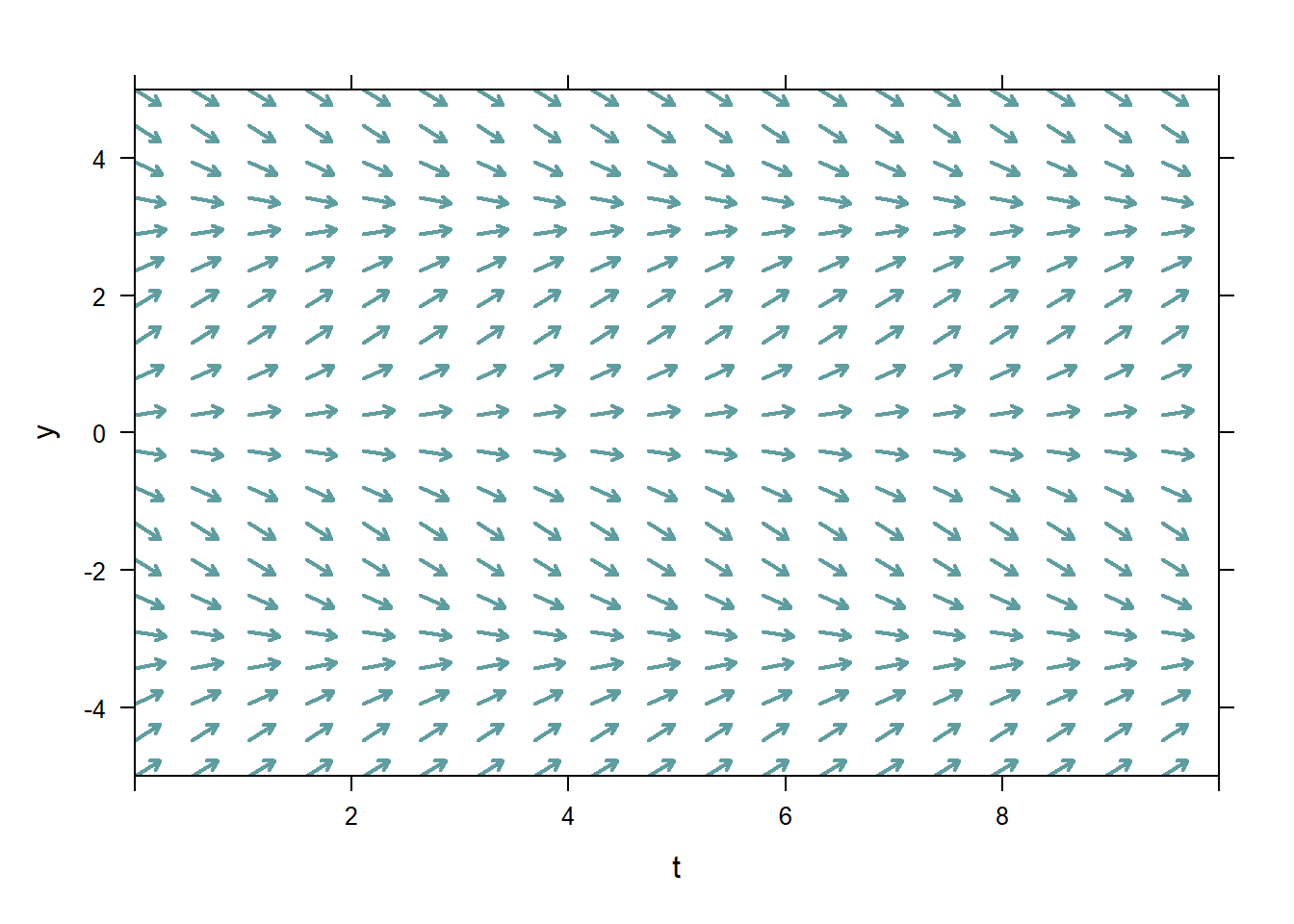
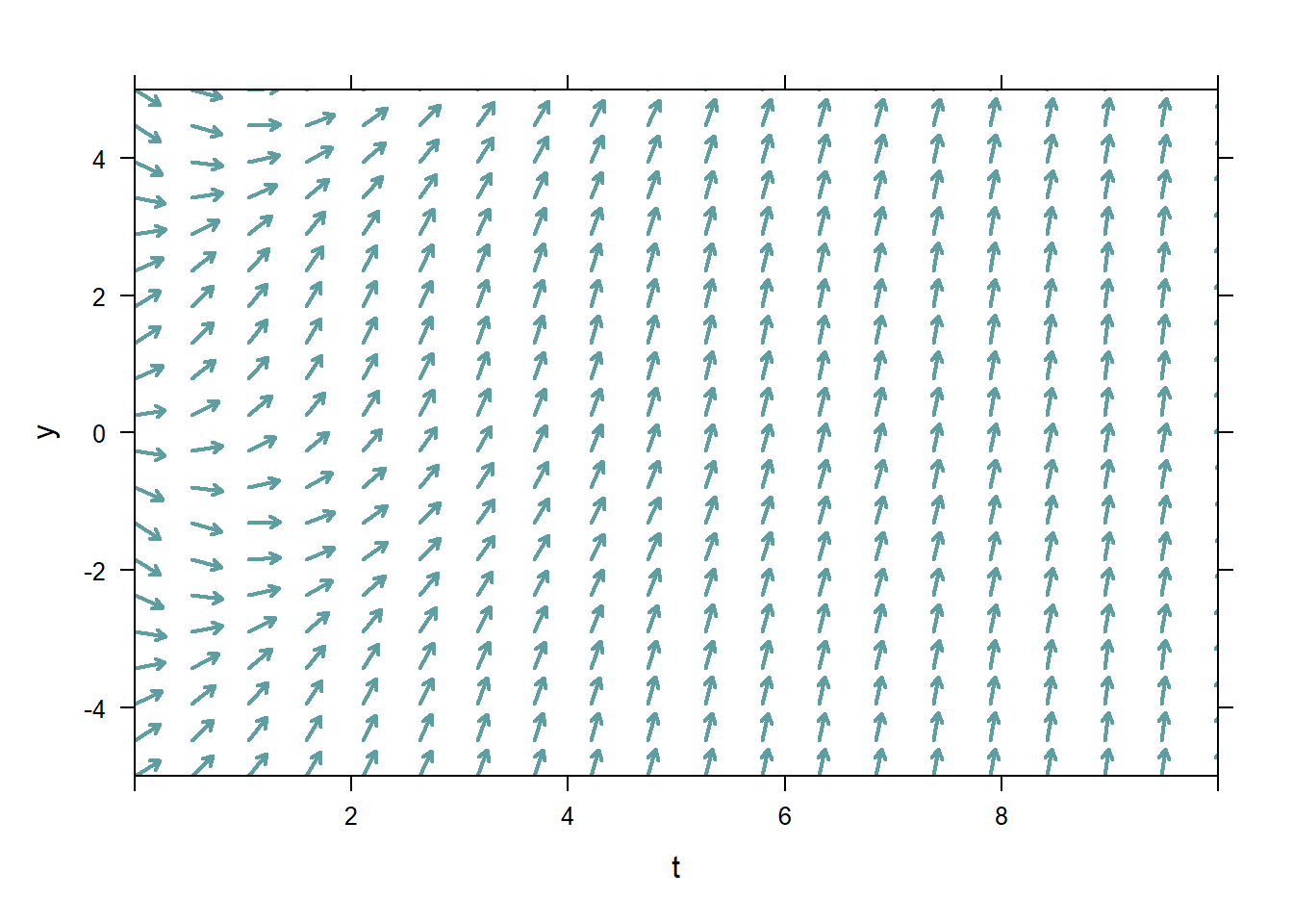
Figure 5.2: Autonomous and non-autonomous ODE direction fields

5.2.0.1 Example #1

Create the direction field using this ODE

$$y^{'} = e^{- t}\cos(4t)\ \ \text{ for}\ \ -2 \leq t \leq 3\ \text{ and}\ - 2 \leq y \leq 3.$$ Is this differential equation autonomous, pure-time, or neither? What should its direction field look like?

Once you have plotted the direction field, plot solutions for the following ICs: $(-2,0)$, $(-2,2)$, and $(-2, - 1)$.

Solution

plotODEDirectionField(exp(-t)*cos(4*t)~t&y,tlim=c(-2,3),ylim=c(-2,3),ics=c(0,2,-1))

This differential equation is pure-time, because $y'$ depends only on $t$, not on $y$. We can see that the direction field for the ODE does not vary in the $y$-direction.

5.2.0.2 Example #2

Create the direction field using this ODE

$$y^{'} = y+\frac{1}{1+t^2}\ \ \text{ for}\ \ -5 \leq t \leq 5\ \text{ and}\ - 5 \leq y \leq 5$$ Is this differential equation autonomous, pure-time, or neither? What does this tell us about its direction field?

Plot solutions for the following ICs: $(-5,0)$, $(-5,2)$, and $(-5, -1)$.

Solution

plotODEDirectionField(y+1/(1+t^2)~t&y,tlim=c(-5,5),ylim=c(-5,5),ics=c(0,2,-1))

This differential equation is neither autonomous nor pure-time, since $y'$ depends on both $y$ and $t$. The direction field for the ODE varies in both the $y$- and $t$-directions.

5.2.0.3 Example #3

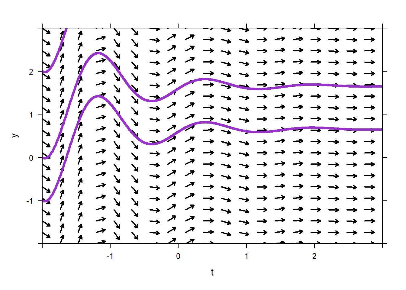
Here is a direction field. Which of the ODEs below does it correspond to?

	Possible ODEs
#1	$$y^{'} = \sin(t) - 1$$
#2	$$y^{'} = y^2$$
#3	$$y^{'} = -y$$

First, we can see that the direction field does not vary in the $t$-direction, so the corresponding ODE must be autnonomous. Therefore, the direction field does not correspond to #1.

Next, we can pick a specific point on the direction field, and see if we can eliminate any options. For example, consider the point $(t=-2,y=1)$.

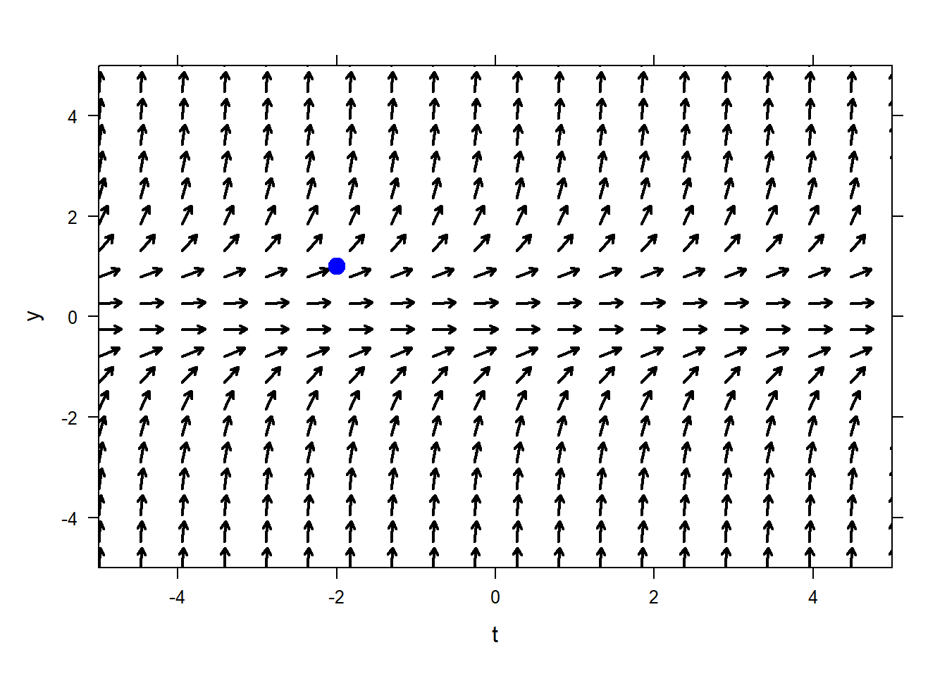If we were to draw a direction field for option 2, the vector emanating from $(-2,1)$ would have slope $1^2=1$, which is positive. That is consistent with the direction field we have. On the other hand, if were were to draw a direction field for option 3, the vector emanating from $(-2,1)$ would have slope $-(1)=-1$ which is negative; that is not consistent with the direction field we have. Therefore we can eliminate option 3 as a possibility and conclude that the direction field must correspond to option 2.

5.3 Exercises

Problems 1) – 4). Using plotODEDirectionField, complete 3 steps: a) plot the direction field, b) plot the solutions linked to the given ICs, and c) discuss your results.

	ODE	$\mathbf{t}$ domain	$\mathbf{y}$ range	ICs
1)	$$y^{'} = t$$	$$0 \leq t \leq 5$$	$$0 \leq y \leq 10$$	$(0,\ 0);$ $(0,\ 2)$; $(0,\ 7)$
2)	$$y^{'} = \cos(y)$$	$$0 \leq t \leq 10$$	$$- 2 \leq y \leq 2$$	$(0, - 1);$ $(0,\ 0)$; $(0,\ 1)$
3)	$$y^{'} = 0$$	$$- 5 \leq t \leq 5$$	$$- 5 \leq y \leq 5$$	$(0, - 4);$ $(0, - 2)$; $(0,\ 3)$
4)	$$y^{'} = e^{- t-y}$$	$$- 2 \leq t \leq 2$$	$$- 5 \leq y \leq 5$$	$( - 2,\ - 5);$ $(0,\ - 5)$; $( - 1,\ - 1)$

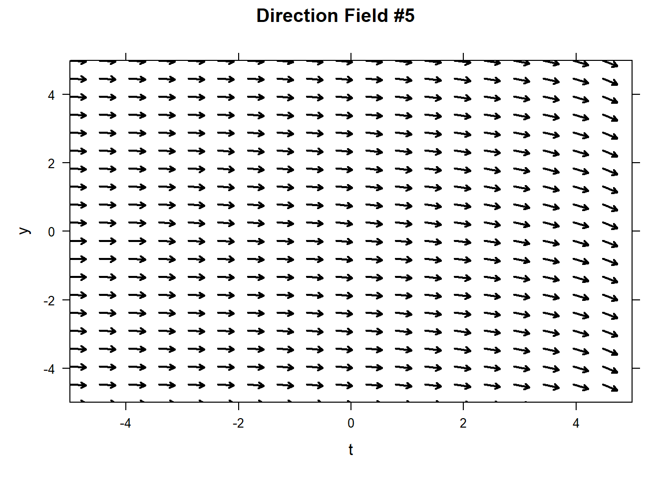
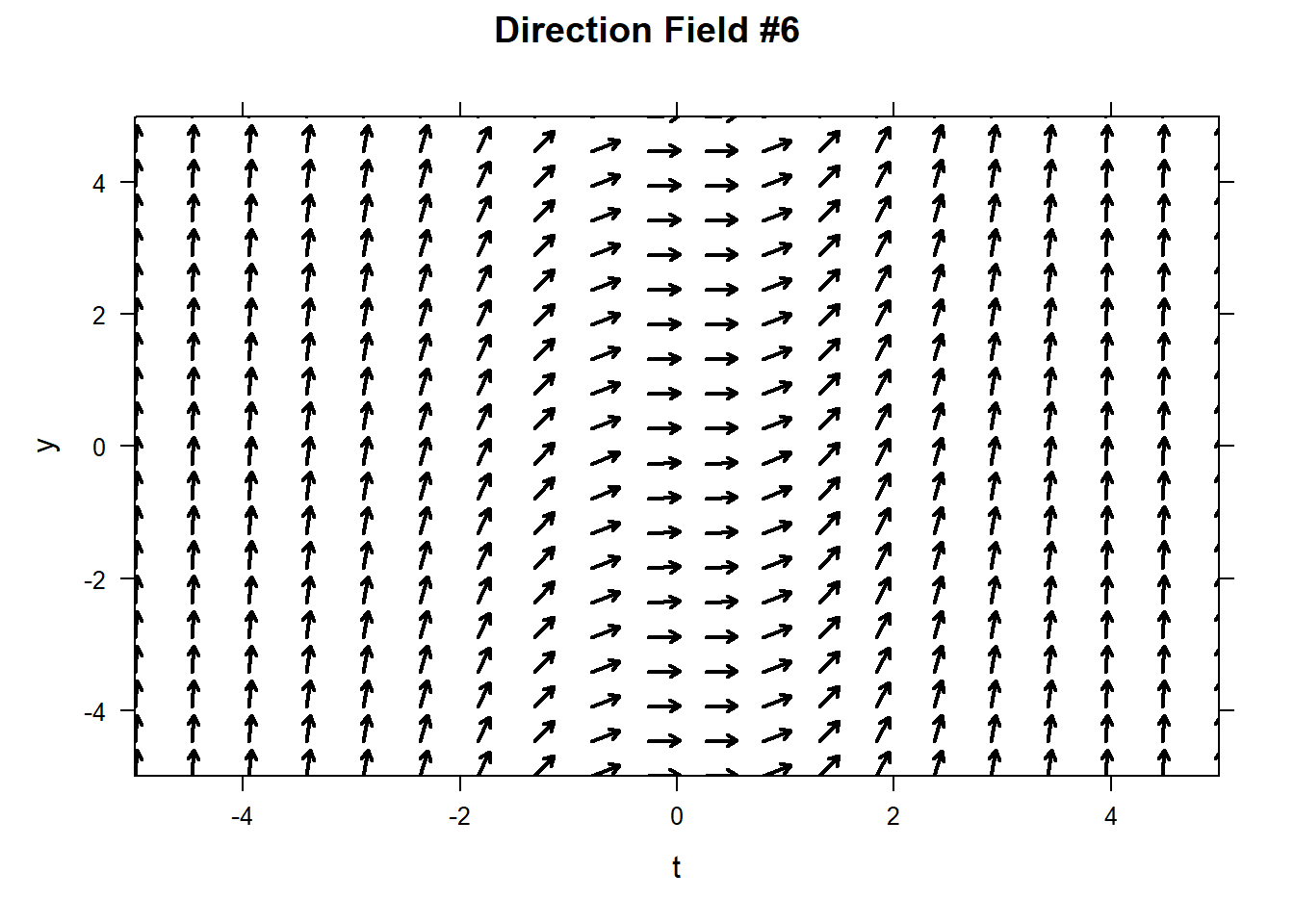
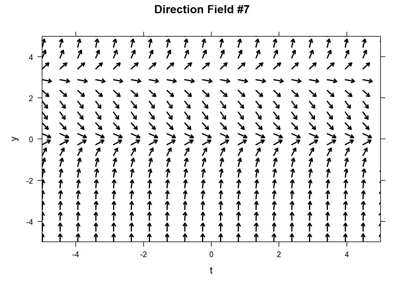
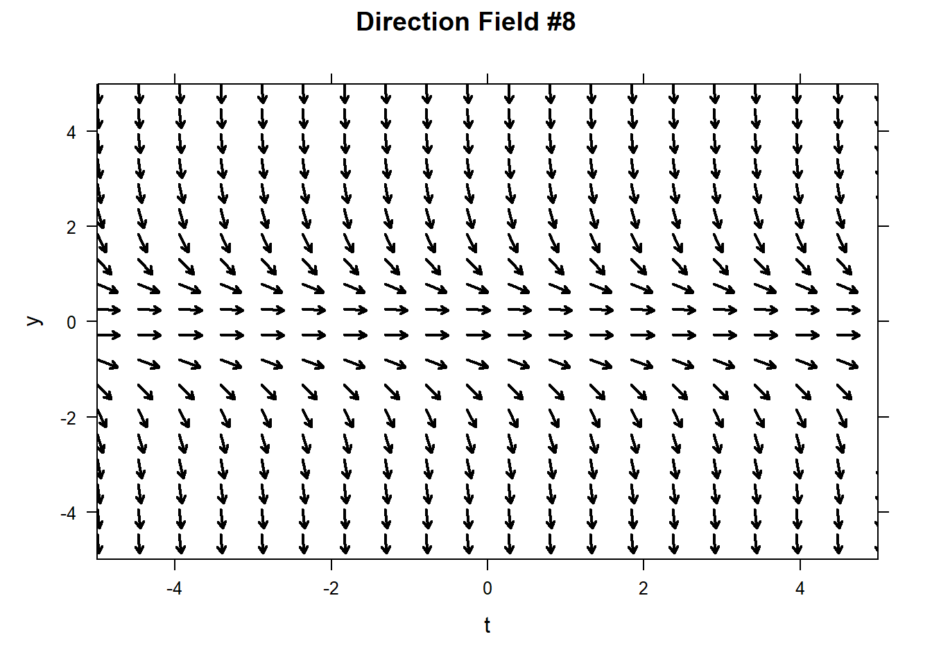
Problems 5) – 12). Match each differential equation with its direction field. For each direction field sketch the solution associated with the given initial condition.

ODE	Direction Field	ODE	Direction Field
$$y^{'} = \frac{1}{t - 6}$$	#________	$$y^{'} = - 1$$	#________
$$y^{'} = -y^2$$	#________	$$y^{'} = y$$	#________
$$y^{'} = \sin(t+y)$$	#________	$$y^{'} =y(y-3)$$	#________
$$y^{'} = t^2$$	#________	$$y^{'} = \cos(t) - 1$$	#________